A virus spreads in a lab sample, medicine leaves the bloodstream, and an investment grows continuously. These situations look very different, but mathematically they often lead to the same challenge: the variable is trapped in an exponent. When that happens, subtraction and division are no longer enough. To unlock the exponent, we use one of algebra's most powerful tools: the logarithm.
In many equations, the variable is multiplied by a number, so you can isolate it with inverse operations. For example, if \(5t=20\), then dividing by \(5\) gives \(t=4\). But in an equation like \(2^t=20\), the variable \(t\) is an exponent. There is no basic arithmetic operation that removes an exponent directly. That is why we need a logarithm.
A logarithm answers a question like this: "To what exponent must a base be raised to get a certain number?" For example, \(\log_2 8=3\) because \(2^3=8\). This inverse relationship between exponents and logarithms is the key idea of the whole lesson.
When solving equations, always try to isolate the part containing the variable. In an exponential equation, that usually means getting the expression with the exponent by itself before applying a logarithm.
For exponential models, the equation often appears in the form \(ab^{ct}=d\). This form is common in science, finance, and population studies because constants can rescale the initial value and stretch or compress time.
Let us look closely at the equation \(ab^{ct}=d\). Here, \(a\), \(c\), and \(d\) are numbers, \(b\) is the base, and in this lesson the base is one of \(2\), \(10\), or \(e\). The variable is \(t\), usually representing time.
Each part has a role. The number \(a\) is a scale factor, often the initial amount. The base \(b\) determines the kind of growth or decay. The number \(c\) changes how fast the exponent grows with time. The number \(d\) is the target value you want to reach.
An exponential model is a model in which a quantity changes by equal factors over equal intervals, often written in a form such as \(y=ab^{x}\) or \(y=ae^{kt}\).
Natural logarithm is the logarithm with base \(e\), written as \(\ln x\).
To solve \(ab^{ct}=d\), the first goal is to isolate the exponential expression. If \(a\neq 0\), divide both sides by \(a\):
\[b^{ct}=\frac{d}{a}\]
Now the variable is still in the exponent, but the equation is in a form where logarithms can help. At this stage, a real solution is only possible if \(\dfrac{d}{a}>0\), because the bases \(2\), \(10\), and \(e\) raised to any real power always produce positive values.
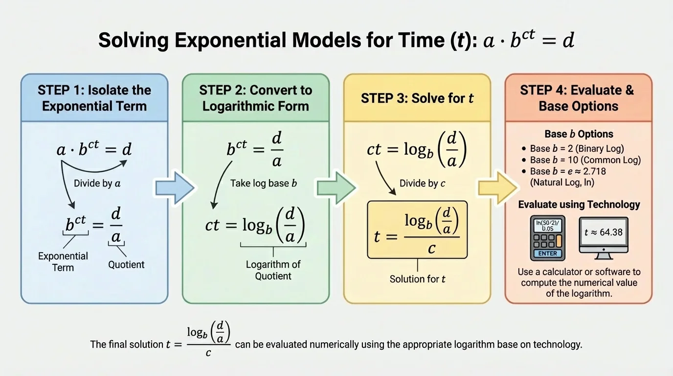
[Figure 1] outlines the conversion process from the original exponential equation to a logarithmic equation and then to a direct expression for \(t\). Starting from \(b^{ct}=\dfrac{d}{a}\), apply a logarithm with base \(b\) to both sides. Because logarithms undo exponents, you get \(ct=\log_b\left(\dfrac{d}{a}\right)\).
Now divide both sides by \(c\), as long as \(c\neq 0\):
\[t=\frac{\log_b\left(\frac{d}{a}\right)}{c}\]
This is the general solution for equations of the form \(ab^{ct}=d\). It is often the cleanest exact answer, especially when the target value is not a perfect power of the base.
You can also think about this conversion using equivalent forms. If \(b^x=y\), then \(x=\log_b y\). In our equation, the exponent is not just \(t\); it is \(ct\). That is why the logarithm gives \(ct\) first, and only after that do we divide by \(c\).
Why the formula works
Exponential and logarithmic functions are inverses. That means they undo each other. If \(b^x=y\), then \(\log_b y=x\). In \(ab^{ct}=d\), dividing by \(a\) isolates the exponential part, and the logarithm reveals the exponent \(ct\). This is the same inverse idea you use when square roots undo squaring.
As a quick check, notice that if \(\dfrac{d}{a}=1\), then \(\log_b 1=0\), so \(t=0\). That makes sense because \(b^0=1\), so the equation becomes \(a=d\).
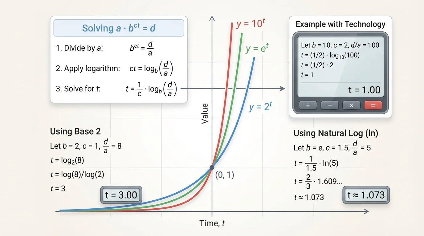
Different exponential models use different bases, and those bases produce different growth patterns, as [Figure 2] illustrates. In this lesson, the most important bases are \(2\), \(10\), and \(e\).
If the base is \(2\), then the solution is written with \(\log_2\). If the base is \(10\), we usually write \(\log\), which means the common logarithm, or logarithm base \(10\). If the base is \(e\), we write \(\ln\), the natural logarithm.
So the three forms are:
\[t=\frac{\log_2\left(\frac{d}{a}\right)}{c}\]
\[t=\frac{\log\left(\frac{d}{a}\right)}{c}\]
\[t=\frac{\ln\left(\frac{d}{a}\right)}{c}\]
On many calculators, there is no \(\log_2\) button. Technology often provides \(\log\) and \(\ln\) keys. In that case, use the change-of-base formula:
\[\log_2 x=\frac{\log x}{\log 2}=\frac{\ln x}{\ln 2}\]
This means any logarithm with base \(2\) can still be evaluated with standard technology. For example, \(\log_2 7\) can be entered as \(\dfrac{\log 7}{\log 2}\) or \(\dfrac{\ln 7}{\ln 2}\).
Because base \(10\) and base \(e\) are built directly into most calculators, equations using those bases are usually easiest to evaluate numerically. Still, the underlying method is identical for all three bases.
Example 1: Base \(2\)
Solve \(3\cdot 2^{4t}=50\).
Step 1: Isolate the exponential expression.
Divide both sides by \(3\): \(2^{4t}=\dfrac{50}{3}\).
Step 2: Rewrite in logarithmic form.
Since the base is \(2\), \(4t=\log_2\left(\dfrac{50}{3}\right)\).
Step 3: Solve for \(t\).
Divide by \(4\): \(t=\dfrac{\log_2(50/3)}{4}\).
Step 4: Evaluate with technology.
Using change of base, \(t=\dfrac{1}{4}\cdot \dfrac{\log(50/3)}{\log 2}\approx \dfrac{1}{4}(4.0589)\approx 1.0147\).
\[t\approx 1.015\]
This answer means the model reaches \(50\) units a little after \(t=1\). Exact form and approximate form are both useful: the logarithm gives precision, and the decimal gives practical meaning.
Example 2: Base \(10\)
Solve \(5\cdot 10^{0.3t}=80\).
Step 1: Isolate the power of \(10\).
Divide by \(5\): \(10^{0.3t}=16\).
Step 2: Apply base-\(10\) logarithm.
\(0.3t=\log 16\).
Step 3: Solve for \(t\).
\(t=\dfrac{\log 16}{0.3}\).
Step 4: Evaluate.
Since \(\log 16\approx 1.2041\), \(t\approx \dfrac{1.2041}{0.3}\approx 4.0137\).
\[t\approx 4.014\]
Notice how convenient base \(10\) is on a calculator. You can enter the expression directly with the \(\log\) key.
Example 3: Base \(e\)
Solve \(12e^{1.5t}=100\).
Step 1: Isolate the exponential factor.
Divide by \(12\): \(e^{1.5t}=\dfrac{100}{12}=\dfrac{25}{3}\).
Step 2: Apply natural logarithm.
\(1.5t=\ln\left(\dfrac{25}{3}\right)\).
Step 3: Solve for \(t\).
\(t=\dfrac{\ln(25/3)}{1.5}\).
Step 4: Evaluate.
\(\ln(25/3)\approx 2.1203\), so \(t\approx \dfrac{2.1203}{1.5}\approx 1.4135\).
\[t\approx 1.414\]
Exponential models with base \(e\) appear often in advanced science because continuous growth and continuous decay are naturally modeled by \(e^{kt}\).
Example 4: Negative \(c\) in a decay model
Solve \(200e^{-0.4t}=35\).
Step 1: Isolate the exponential part.
Divide by \(200\): \(e^{-0.4t}=0.175\).
Step 2: Apply \(\ln\).
\(-0.4t=\ln(0.175)\).
Step 3: Solve for \(t\).
\(t=\dfrac{\ln(0.175)}{-0.4}\).
Step 4: Evaluate.
Since \(\ln(0.175)\approx -1.7430\), \(t\approx \dfrac{-1.7430}{-0.4}\approx 4.3575\).
\[t\approx 4.358\]
This example is important because students sometimes worry when the logarithm is negative. That is not a problem. In fact, decay models often produce a negative logarithm, and dividing by a negative rate can still lead to a positive time value.
There are several details that matter when solving equations of the form \(ab^{ct}=d\). First, you must divide by \(a\) before applying the logarithm, unless the equation is already isolated. Forgetting that step is one of the most common errors.
Second, the quantity inside the logarithm must be positive. In the formula \(t=\dfrac{\log_b(d/a)}{c}\), the expression \(\dfrac{d}{a}\) must satisfy \(\dfrac{d}{a}>0\). If \(\dfrac{d}{a}\leq 0\), then there is no real solution.
Third, make sure the denominator \(c\) is not \(0\). If \(c=0\), then the equation becomes \(ab^0=d\), which simplifies to \(a=d\). In that special case, either every value of \(t\) works or no value does, depending on whether \(a=d\).
Many calculators use the key labels log for base \(10\) and ln for base \(e\). Some graphing apps also allow you to type \(logBASE(value)\), but the exact syntax depends on the device.
Another common mistake is mixing up exact and approximate answers. The expression \(\dfrac{\ln(25/3)}{1.5}\) is exact. The decimal \(1.414\) is an approximation. In modeling, decimals are often necessary, but it is still useful to know the exact logarithmic form.
The relationship between bases still matters later, as we saw in [Figure 2], because a larger base can lead to faster growth for the same exponent pattern. Even when the algebraic method stays the same, the model's behavior changes with the base.
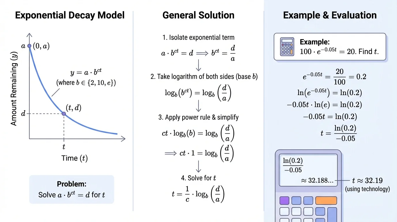
[Figure 3] shows why exponential models are powerful: they describe repeated multiplication. In growth situations, a quantity increases by the same factor over equal time intervals. In decay situations, it decreases by the same multiplicative factor over equal time intervals. A graph of decay drops quickly at first and then levels off.
Suppose a medicine in the bloodstream is modeled by \(A=150e^{-0.2t}\), where \(A\) is the amount in milligrams after \(t\) hours. To find when only \(40\) milligrams remain, solve \(150e^{-0.2t}=40\). Then \(e^{-0.2t}=\dfrac{4}{15}\), so \(t=\dfrac{\ln(4/15)}{-0.2}\approx 6.61\). The logarithm tells you the time when the target amount is reached.
In population studies, a species might follow a model such as \(P=80\cdot 2^{0.5t}\). To find when the population reaches \(500\), solve \(80\cdot 2^{0.5t}=500\). The result is \(t=\dfrac{\log_2(500/80)}{0.5}\). Even if the number is not a whole number of years, the logarithm still gives the precise answer.
In finance, exponential growth may use base \(10\) less often than base \(e\), but the same structure appears whenever a quantity grows by a fixed percent. In chemistry and physics, base \(e\) is especially common because continuously changing rates are modeled naturally with \(e^{kt}\).
Radioactive decay is another strong example. If a sample follows \(N=N_0e^{-kt}\), the time needed to decay to a certain amount is found by taking \(\ln\) and solving for \(t\). That is exactly the same algebra as in the examples above. The curve shape in [Figure 3] matches this kind of process: steep change first, slower change later.
When you solve for \(t\), the answer is usually a time value. But the number only matters if you attach it to the context. A result like \(t\approx 4.014\) could mean \(4.014\) years, \(4.014\) months, or \(4.014\) hours, depending on the model.
It is also important to decide how much rounding makes sense. If a model measures time in seconds, rounding to the nearest thousandth may be reasonable. If the context is a long-term population study, rounding to the nearest tenth or whole number may make more sense.
Whenever possible, check your answer by substitution. For instance, if \(t\approx 1.015\) in the equation \(3\cdot 2^{4t}=50\), substituting gives \(3\cdot 2^{4(1.015)}\approx 3\cdot 16.67\approx 50.01\), which confirms that the solution is sensible.
The transformation path introduced earlier in [Figure 1] is the pattern to remember: isolate the exponential expression, convert to logarithmic form, divide by the coefficient of \(t\), and then evaluate with technology if needed.
| Base | Logarithm notation | Solution form for \(ab^{ct}=d\) | Calculator note |
|---|---|---|---|
| \(2\) | \(\log_2\) | \(t=\dfrac{\log_2(d/a)}{c}\) | Usually use change of base |
| \(10\) | \(\log\) | \(t=\dfrac{\log(d/a)}{c}\) | Use the \(\log\) key |
| \(e\) | \(\ln\) | \(t=\dfrac{\ln(d/a)}{c}\) | Use the \(\ln\) key |
Table 1. Comparison of solution forms and calculator methods for exponential equations with bases \(2\), \(10\), and \(e\).