A streaming service gains the same number of subscribers each month in one city, but in another city the number of subscribers grows by the same percent each month. At first those stories can sound similar, but mathematically they are completely different. One follows a straight-line pattern. The other changes multiplicatively over time. Learning to build the right kind of function from a graph, a table, a verbal description, or just two points lets you turn patterns into equations you can actually use.
Many real situations can be modeled by either a linear function or an exponential function. A linear function represents change by equal amounts over equal intervals. An exponential function represents change by equal factors over equal intervals. That difference—adding versus multiplying—is the central idea of this topic.
These models appear in finance, medicine, engineering, social media analytics, and environmental science. If a car loses the same dollar value each year, a linear model may fit. If a population grows by the same percent each year, an exponential model may fit. The skill is not only solving equations; it is constructing them from information you are given.
Linear function: a function with a constant rate of change. It can often be written as \(y = mx + b\), where \(m\) is the slope and \(b\) is the \(y\)-intercept.
Exponential function: a function with a constant multiplicative rate of change. It can often be written as \(y = ab^x\), where \(a\) is the initial value and \(b\) is the growth or decay factor.
Arithmetic sequence: a sequence with a constant difference between consecutive terms.
Geometric sequence: a sequence with a constant ratio between consecutive terms.
When you decide which model to use, look at how the output changes as the input increases. If the output keeps increasing by something like \(+5\), \(-2\), or \(+0.75\), think linear. If the output keeps multiplying by something like \(1.2\), \(0.8\), or \(3\), think exponential.
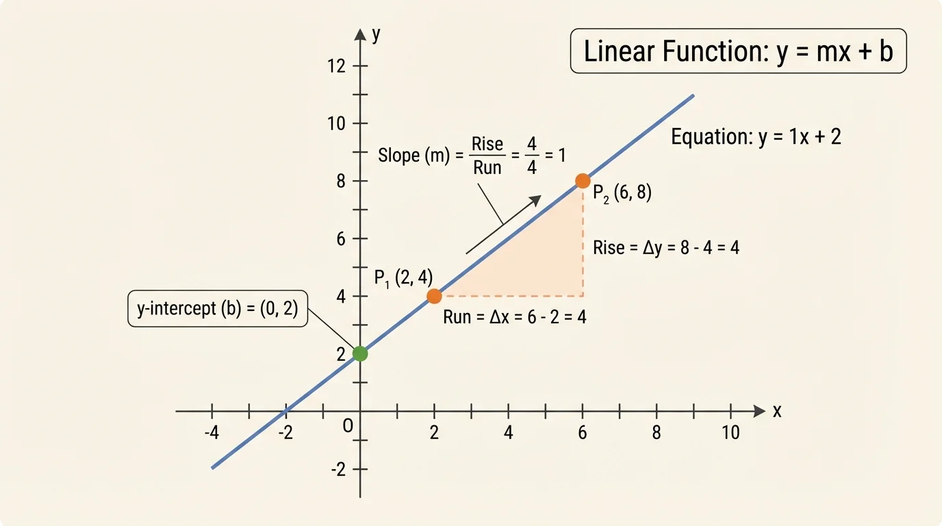
A linear relationship is built on a constant rate of change. If increasing \(x\) by \(1\) always changes \(y\) by \(4\), the slope is \(4\). In general, for two points \((x_1, y_1)\) and \((x_2, y_2)\), the slope is \[m = \frac{y_2-y_1}{x_2-x_1}\]. Once the slope is known, you can write the function in slope-intercept form or point-slope form.
An exponential relationship is built on a constant factor. If increasing \(x\) by \(1\) always multiplies \(y\) by \(1.5\), then the factor is \(1.5\). If it multiplies by \(0.7\), the quantity is decaying. In the form \(y = ab^x\), \(a\) is the value when \(x = 0\), and \(b\) is the repeated multiplier.
From earlier algebra, you already know how to substitute values into equations and solve for unknowns. You also know that a point \((x, y)\) means the input is \(x\) and the output is \(y\). Those ideas are essential here.
Sequences fit naturally into this topic because a sequence is a function whose inputs are term numbers such as \(1, 2, 3, 4, ...\). An arithmetic sequence behaves like a linear function. A geometric sequence behaves like an exponential function.
To construct a linear function, identify the constant additive change. On a graph, this appears as the same rise over run between any two points, as [Figure 1] shows. In a table, the first differences are constant. In a verbal description, look for phrases such as "increases by \(3\) each hour" or "starts at \(50\) and drops \(4\) per day."
If you know two points, find the slope first. Then substitute one point into \(y = mx + b\) to find \(b\). If the information comes from a table, you can use any two rows as long as the relationship is linear.
Suppose a table gives the points \((1, 7)\), \((3, 13)\), and \((5, 19)\). The output changes by \(+6\) when the input changes by \(+2\), so the slope is \(\dfrac{6}{2} = 3\). Using \((1, 7)\), we get \(7 = 3(1) + b\), so \(b = 4\). The function is \(y = 3x + 4\).
Descriptions can be translated directly. If a gym charges a \$25\ sign-up fee and then \$15\ per month, the starting amount is \$25\ and the rate is \(15\) dollars per month. Letting \(x\) be months and \(y\) be total cost, the function is \(y = 15x + 25\).
Worked example 1: linear function from two input-output pairs
Construct the linear function passing through \((2, 11)\) and \((6, 23)\).
Step 1: Find the slope.
Use \(m = \dfrac{y_2-y_1}{x_2-x_1}\): \(m = \dfrac{23-11}{6-2} = \dfrac{12}{4} = 3\).
Step 2: Substitute into \(y = mx + b\).
Use the point \((2, 11)\): \(11 = 3(2) + b\), so \(11 = 6 + b\), and therefore \(b = 5\).
Step 3: Write the function.
The linear function is \(y = 3x + 5\).
A quick check with \(x = 6\) gives \(y = 3(6) + 5 = 23\), which matches the second point.
Another useful form is point-slope form: \(y - y_1 = m(x - x_1)\). Using the same points, you could write \(y - 11 = 3(x - 2)\). Expanding leads back to \(y = 3x + 5\).
To construct an exponential function, identify the constant multiplicative change. Equal steps in the input produce outputs that are multiplied by the same number. In a table, check whether consecutive outputs have a common ratio. In a description, look for phrases such as "grows by \(8\%\) each year," "triples every hour," or "retains \(90\%\) of its value each year."
[Figure 2] In the form \(y = ab^x\), \(a\) is the value at \(x = 0\). The base \(b\) is the growth factor if \(b > 1\) and the decay factor if \(0 < b < 1\). A growth rate of \(12\%\) means \(b = 1.12\). A decay rate of \(12\%\) means \(b = 0.88\).
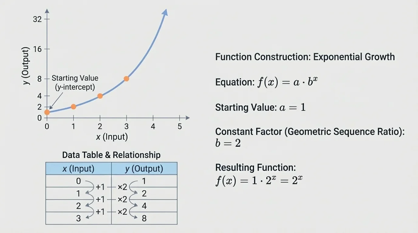
If a table shows \((0, 5)\), \((1, 10)\), \((2, 20)\), and \((3, 40)\), each output is multiplied by \(2\). Since the value at \(x = 0\) is \(5\), the function is \(y = 5 \cdot 2^x\).
If you are given two points and know the relationship is exponential, substitute them into \(y = ab^x\). Often one point lets you find \(a\), and the second lets you find \(b\). This is especially convenient when one point has \(x = 0\).
Worked example 2: exponential function from two input-output pairs
Construct the exponential function passing through \((0, 6)\) and \((3, 48)\).
Step 1: Use the point with \(x = 0\) to find \(a\).
In \(y = ab^x\), substituting \((0, 6)\) gives \(6 = ab^0 = a\). So \(a = 6\).
Step 2: Use the second point to find \(b\).
Substitute \((3, 48)\): \(48 = 6b^3\). Then \(8 = b^3\), so \(b = 2\).
Step 3: Write the function.
The exponential function is \[y = 6 \cdot 2^x\].
Check: when \(x = 3\), \(y = 6 \cdot 2^3 = 6 \cdot 8 = 48\).
When the two given points do not include \(x = 0\), you can still solve by substitution, but the algebra may be more involved. At this level, many construction problems are designed so the ratio is visible from the table or one point gives the initial value directly.
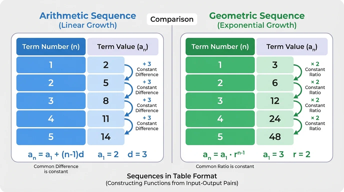
[Figure 3] A sequence can be written as a function of the term number, and the two main types can be compared naturally. If the first term is \(a_1\), an arithmetic sequence with common difference \(d\) has the explicit rule \[a_n = a_1 + (n-1)d\]. A geometric sequence with common ratio \(r\) has the explicit rule \[a_n = a_1 r^{n-1}\].
Arithmetic sequences are closely connected to linear functions because they add the same amount each step. Geometric sequences are closely connected to exponential functions because they multiply by the same factor each step.
For example, the arithmetic sequence \(4, 7, 10, 13, ...\) has first term \(4\) and difference \(3\). Its explicit rule is \(a_n = 4 + (n-1)3\), which simplifies to \(a_n = 3n + 1\).
The geometric sequence \(5, 15, 45, 135, ...\) has first term \(5\) and ratio \(3\). Its explicit rule is \(a_n = 5 \cdot 3^{n-1}\).
Worked example 3: arithmetic sequence from a table
A table shows term numbers \(1, 2, 3, 4\) with outputs \(12, 9, 6, 3\). Construct the explicit rule.
Step 1: Find the common difference.
The terms change by \(-3\) each time, so \(d = -3\).
Step 2: Identify the first term.
The first term is \(a_1 = 12\).
Step 3: Use the arithmetic sequence formula.
\(a_n = a_1 + (n-1)d = 12 + (n-1)(-3)\).
Step 4: Simplify.
\(a_n = 12 - 3n + 3 = 15 - 3n\).
The explicit rule is \[a_n = 15 - 3n\].
Some courses also use recursive rules. For the arithmetic sequence above, a recursive rule is \(a_1 = 12\) and \(a_n = a_{n-1} - 3\). For the geometric sequence \(5, 15, 45, 135, ...\), a recursive rule is \(a_1 = 5\) and \(a_n = 3a_{n-1}\).
Graphs provide visual clues. A straight-line graph indicates a linear function. A curved graph that rises or falls more dramatically over time suggests an exponential function. The visual shape matters, but you still need numerical information from points or intercepts to write the equation exactly.
For a line, identify two clear points. Then compute slope using rise over run, just as in [Figure 1]. If the graph crosses the \(y\)-axis at \(b\), then \(b\) is the intercept in \(y = mx + b\).
For an exponential graph, find the value when \(x = 0\). That is \(a\) in \(y = ab^x\). Then compare outputs for equal increases in \(x\). If each step multiplies by \(b\), that value is the base. This repeated multiplication pattern is the key feature shown earlier in [Figure 2].
Many viruses, investments, and online trends grow approximately exponentially only for a limited time. Real systems eventually hit limits, but exponential models are still extremely powerful for describing early growth.
If a graph is imperfect or points are hard to read exactly, use the clearest labeled points available. In applied settings, a model may be approximate rather than exact.
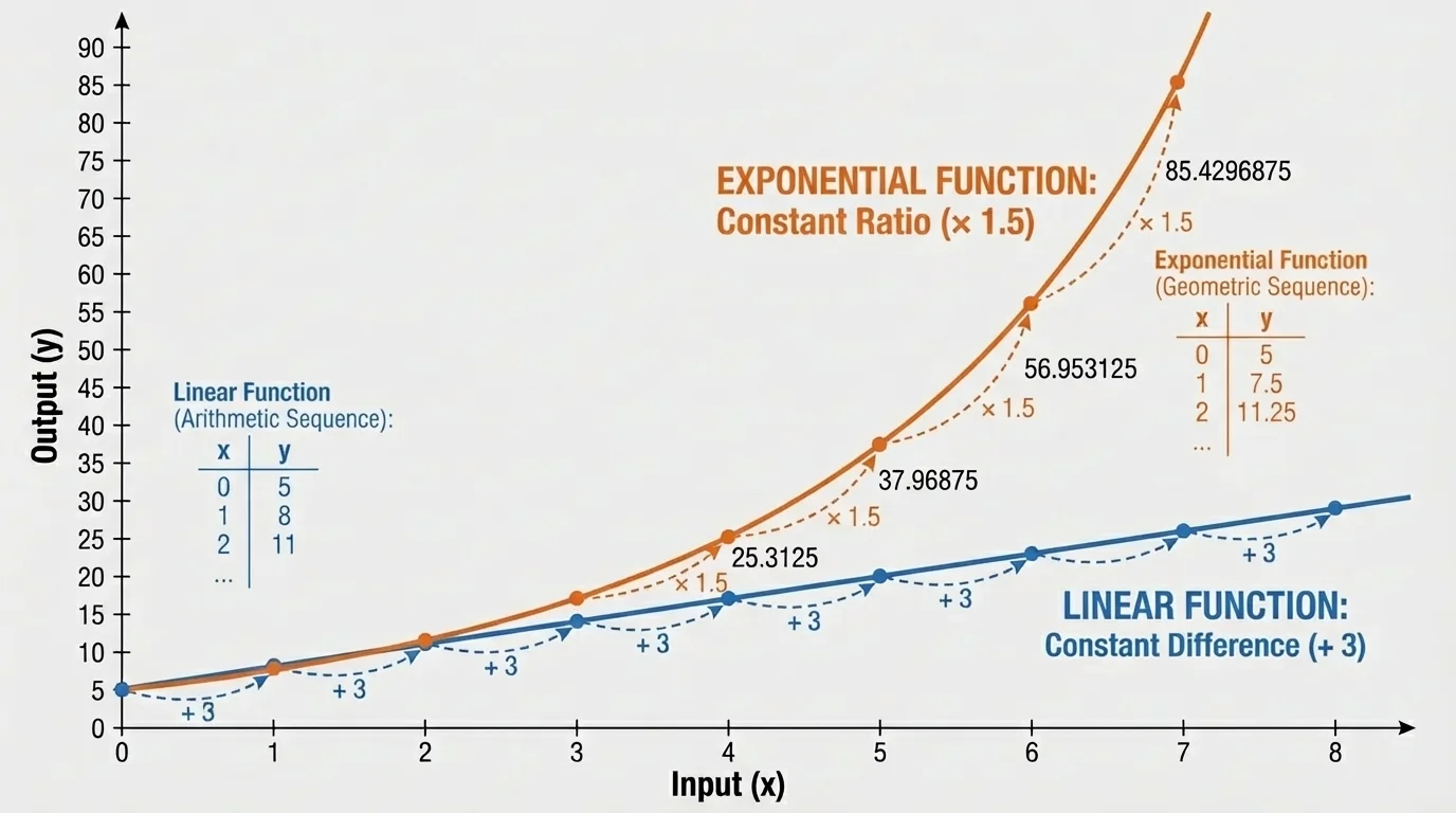
The fastest way to distinguish the models is to examine what stays constant. The overall shapes make the difference visible: a line has constant additive change, while an exponential curve has constant multiplicative change.
| Feature | Linear | Exponential |
|---|---|---|
| General form | \(y = mx + b\) | \(y = ab^x\) |
| Constant pattern | Difference | Ratio |
| Graph shape | Straight line | Curve |
| Table test | Equal first differences | Equal ratios |
| Sequence type | Arithmetic | Geometric |
Table 1. Comparison of linear and exponential models.
[Figure 4] Suppose a table has outputs \(2, 5, 8, 11\). The first differences are \(+3, +3, +3\), so it is linear. If another table has outputs \(2, 6, 18, 54\), the ratios are \(\dfrac{6}{2} = 3\), \(\dfrac{18}{6} = 3\), and \(\dfrac{54}{18} = 3\), so it is exponential.
A common mistake is to see rapid increase and assume exponential immediately. Rapid increase can still be linear if the same amount is added each time. Always test the pattern numerically.
Worked example 4: geometric sequence from a description
A lab culture begins with \(200\) bacteria and doubles every hour. Write an explicit rule for the number of bacteria after \(n\) hours.
Step 1: Identify the initial amount.
At hour \(0\), there are \(200\) bacteria, so the initial value is \(200\).
Step 2: Identify the growth factor.
"Doubles" means multiply by \(2\), so the factor is \(2\).
Step 3: Write the rule.
Since this is exponential growth, use \(y = ab^x\). Letting \(n\) be hours, the rule is \[B(n) = 200 \cdot 2^n\]
After \(4\) hours, \(B(4) = 200 \cdot 2^4 = 200 \cdot 16 = 3{,}200\).
Linear and exponential models are not just classroom patterns. They help predict, compare, and interpret real systems.
Salary plans: If a job offers a starting salary of \$40,000\ and raises it by \$1,500\ each year, the salary follows a linear model. If another investment account grows by \(5\%\) each year, it follows an exponential model. Those two situations may look similar at first, but after enough years, the exponential growth can overtake the linear one.
Depreciation: A device that loses \$80\ of value each year can be modeled linearly. A car that retains \(85\%\) of its value each year is modeled exponentially by multiplying by \(0.85\) repeatedly.
Science and medicine: Drug concentration in the body often decreases exponentially over time. Some cooling and radioactive decay processes also follow exponential patterns. On the other hand, a machine producing the same number of parts each hour fits a linear model.
Data trends: Early social-media growth can appear exponential when shares trigger more shares. A steady increase in users from a marketing campaign may be closer to linear. This comparison helps explain why long-term predictions can differ dramatically depending on the model chosen.
Mixing up difference and ratio: If you only look at whether numbers are getting bigger, you can misclassify the model. Check whether the outputs change by a constant difference or a constant ratio.
Using the wrong initial value: In \(y = ab^x\), the value of \(a\) is the output when \(x = 0\), not always the first number listed in a table unless the first input is actually \(0\).
Forgetting input spacing: If the input values in a table go \(0, 2, 4, 6\), then each step is an increase of \(2\), not \(1\). Your difference or ratio must be interpreted over equal input intervals.
Confusing sequence notation and function notation: For sequences, \(a_n\) means the \(n\)-th term. For functions, you may see \(f(x)\) or \(y\). The ideas are connected, but the notation tells you how the relationship is being presented.
How to choose the model quickly
Ask two questions. First: when the input increases by equal amounts, does the output change by equal differences or equal factors? Second: does the graph look straight or curved? If the pattern is additive and straight, use a linear model. If the pattern is multiplicative and curved, use an exponential model. Arithmetic sequences match linear thinking, and geometric sequences match exponential thinking.
Constructing functions is really about reading structure. You move between words, tables, points, graphs, and equations, but the underlying pattern stays the same. When you can recognize that structure, you can model unfamiliar situations with confidence.