Some of the most important curves in science, engineering, and economics are polynomial graphs. A ball launched through the air, the approximate shape of a suspension bridge cable over short intervals, and models for revenue or profit can all involve equations whose graphs rise, fall, cross axes, and turn in revealing ways. When a polynomial is written in a useful form, you can often predict major features of its graph before plotting many points.
A polynomial function is built from powers of x that are whole numbers, combined using addition, subtraction, and multiplication. Examples include \(f(x) = 3x^4 - 2x^2 + 7\) and \(g(x) = -2x^3 + 5x - 1\). Non-examples include \(\dfrac{1}{x}\), \(\sqrt{x}\), and \(2^x\), because those do not use only nonnegative integer exponents on x.
Polynomial graphs are smooth and continuous. They have no sharp corners, breaks, or holes. That smoothness means you can often describe the whole graph from a few key pieces of information: its degree, its leading coefficient, its zeros, and sometimes a convenient extra point such as the y-intercept.
Polynomial function is a function of the form \(a_nx^n + a_{n-1}x^{n-1} + \cdots + a_1x + a_0\), where the exponents are whole numbers and the coefficients are real numbers.
Degree is the highest exponent of \(x\) with a nonzero coefficient.
Leading coefficient is the coefficient of the highest-degree term.
The degree helps tell you how many turns the graph can make and how its ends behave far to the left and right. The leading coefficient helps determine whether those ends point upward or downward.
For example, in \(f(x) = -4x^5 + 2x^2 - 7\), the degree is \(5\) and the leading coefficient is \(-4\). Those two pieces already tell you a lot about the graph's long-run behavior.
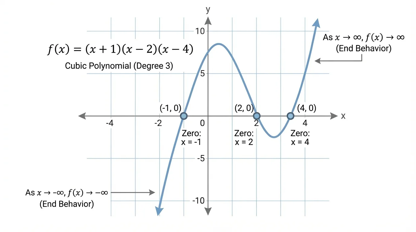
A zero of a polynomial is a value of \(x\) that makes the function equal to \(0\). On the graph, zeros appear where the curve meets the x-axis. When a polynomial is written in factored form, each factor can reveal a zero directly, as [Figure 1] shows through labeled intercepts on a polynomial graph.
If \(f(x) = (x-2)(x+1)(x-4)\), then the zeros are found by setting each factor equal to \(0\): \(x-2=0\), \(x+1=0\), and \(x-4=0\). So the zeros are \(x=2\), \(x=-1\), and \(x=4\). The corresponding x-intercepts are \((2,0)\), \((-1,0)\), and \((4,0)\).
This connection between factors and graph features is one of the most useful ideas in algebra. If you can factor a polynomial, you can often sketch its graph much faster. A zero tells you where the graph hits the axis, but not yet how it behaves there. For that, you need multiplicity.
If a product is \(0\), then at least one factor must be \(0\). This is the zero-product property, and it is the algebra tool behind finding zeros from factored form.
You can also use the y-intercept to anchor the graph. The y-intercept is found by evaluating the function at \(x=0\). For \(f(x) = (x-2)(x+1)(x-4)\), \(f(0)=(-2)(1)(-4)=8\), so the graph passes through \((0,8)\).
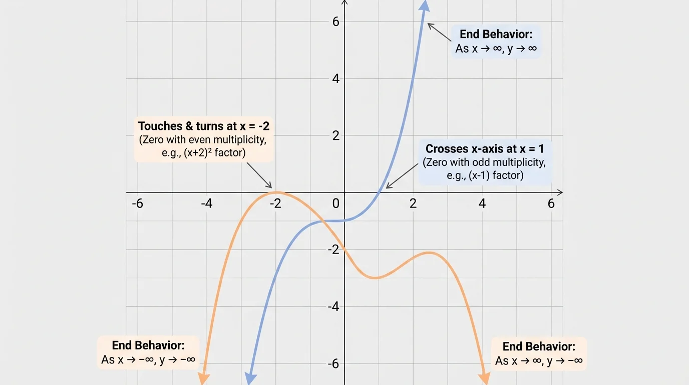
When a factor repeats, the repeated count is called its multiplicity. The graph's local behavior near the zero depends on whether that multiplicity is odd or even, and [Figure 2] makes that difference visible.
If a zero has odd multiplicity, the graph usually crosses the x-axis there. If a zero has even multiplicity, the graph usually touches the axis and turns around, often called "bouncing" off the axis.
For example, consider \(f(x) = (x-3)^2(x+1)\). The zero \(x=3\) has multiplicity \(2\), so the graph touches the axis at \(x=3\) and turns. The zero \(x=-1\) has multiplicity \(1\), so the graph crosses the axis there.
Higher multiplicities can flatten the graph near the axis. For instance, at a zero of multiplicity \(3\), the graph crosses but may look flatter than at a simple zero. At multiplicity \(4\), the graph touches and turns, often with a wider, flatter contact. This flattening matters when you make a careful sketch.
Crossing versus touching
Near a simple zero such as a factor \((x-a)\), the sign of the function changes from positive to negative or from negative to positive, so the graph crosses the axis. Near an even-power factor such as \((x-a)^2\), the expression stays nonnegative or nonpositive on both sides of \(a\), so the graph does not change sign there and instead touches the axis and turns.
This sign-change idea is very powerful. It helps explain why the graph behavior is not random: the algebra in the factor controls the motion of the curve.
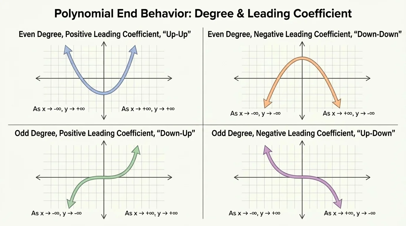
Far to the left and far to the right, the graph of a polynomial is controlled mainly by its highest-degree term. The four standard patterns are organized in [Figure 3], and they depend on whether the degree is odd or even and whether the leading coefficient is positive or negative.
Here is the basic idea:
| Degree | Leading coefficient | Left end | Right end |
|---|---|---|---|
| Even | Positive | Up | Up |
| Even | Negative | Down | Down |
| Odd | Positive | Down | Up |
| Odd | Negative | Up | Down |
Table 1. End behavior patterns for polynomial functions based on degree and leading coefficient.
In symbolic language, if the leading term is \(ax^n\), then for large positive or negative values of \(x\), the function behaves much like \(ax^n\). That is why end behavior can often be determined without factoring the whole polynomial.
For example, if \(f(x) = 2x^4 - 7x + 1\), the degree is \(4\) and the leading coefficient is positive. So as \(x \to -\infty\), \(f(x) \to \infty\), and as \(x \to \infty\), \(f(x) \to \infty\). Both ends go up.
If \(g(x) = -3x^3 + x^2 - 5\), then the degree is \(3\) and the leading coefficient is negative. So as \(x \to -\infty\), \(g(x) \to \infty\), and as \(x \to \infty\), \(g(x) \to -\infty\). The left end goes up and the right end goes down.
Even before graphing calculators existed, mathematicians could predict the general shape of polynomial graphs by using only symbolic clues such as degree, factors, and sign changes. A surprisingly accurate sketch can come from a small amount of algebra.
The patterns in [Figure 3] become especially useful when combined with zeros and multiplicities. End behavior tells you where the graph is heading, while zeros tell you where it must meet the axis on the way.
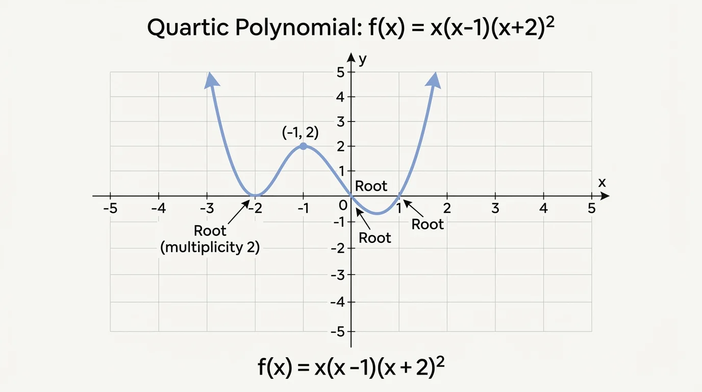
To sketch a polynomial by hand, combine several clues in a logical order. A complete sketch uses end behavior, zeros, multiplicities, and at least one additional point such as the y-intercept. The synthesis of these clues is visible in [Figure 4], where one graph is built from all of them together.
A useful process is:
First, identify the degree and leading coefficient to determine end behavior.
Second, factor the polynomial if possible and find its zeros.
Third, determine the multiplicity of each zero and decide whether the graph crosses or touches the axis there.
Fourth, find the y-intercept by evaluating \(f(0)\).
Fifth, sketch a smooth curve that follows the end behavior and passes through the known intercepts in a way consistent with the multiplicities.
Solved Example 1
Graph \(f(x) = (x-1)(x+2)(x-3)\).
Step 1: Find the zeros.
Set each factor equal to \(0\): \(x-1=0\), \(x+2=0\), and \(x-3=0\). The zeros are \(x=1\), \(x=-2\), and \(x=3\).
Step 2: Identify multiplicities.
Each factor appears once, so each zero has multiplicity \(1\). The graph crosses the x-axis at all three zeros.
Step 3: Determine end behavior.
The polynomial has degree \(3\) with positive leading coefficient \(1\). Therefore the left end goes down and the right end goes up.
Step 4: Find the y-intercept.
\(f(0) = (-1)(2)(-3) = 6\), so the graph passes through \((0,6)\).
Step 5: Sketch the graph.
Start low on the left, cross at \((-2,0)\), pass through \((0,6)\), cross again at \((1,0)\), dip below the axis, then cross at \((3,0)\) and rise to the right.
The key graph features are the intercepts \((-2,0)\), \((1,0)\), \((3,0)\), and \((0,6)\), with odd-degree positive end behavior.
This first example shows the most direct situation: all zeros are simple, so every intercept is a crossing point. In more interesting cases, repeated factors change that behavior.
Solved Example 2
Graph \(g(x) = -(x+1)^2(x-2)\).
Step 1: Find the zeros.
The zeros are \(x=-1\) and \(x=2\).
Step 2: Determine multiplicities.
The factor \((x+1)^2\) gives \(x=-1\) multiplicity \(2\), so the graph touches the axis and turns there. The factor \((x-2)\) gives \(x=2\) multiplicity \(1\), so the graph crosses there.
Step 3: Determine end behavior.
The degree is \(3\). Because of the negative sign in front, the leading coefficient is negative. So the left end goes up and the right end goes down.
Step 4: Find the y-intercept.
\(g(0)=-(1)^2(-2)=2\), so the graph passes through \((0,2)\).
Step 5: Sketch the graph.
Begin high on the left, move down to touch and turn at \((-1,0)\), rise through \((0,2)\), then fall, crossing at \((2,0)\), and continue downward to the right.
This graph combines one bounce and one crossing.
The distinction between touching and crossing in Example 2 matches the pattern shown earlier in [Figure 2]. Repeated factors matter just as much as the zeros themselves.
Solved Example 3
Analyze and sketch \(h(x) = x^2(x-4)^2\).
Step 1: Find the zeros.
From the factors, the zeros are \(x=0\) and \(x=4\).
Step 2: Determine multiplicities.
Both zeros have multiplicity \(2\). The graph touches and turns at both \(x=0\) and \(x=4\).
Step 3: Determine end behavior.
The degree is \(4\) and the leading coefficient is positive, so both ends go up.
Step 4: Find additional points.
Since \(h(2)=2^2(2-4)^2=4\cdot 4=16\), the graph passes through \((2,16)\).
Step 5: Sketch the graph.
The graph comes down from above, touches the axis at \((0,0)\), rises, reaches values such as \(16\) at \(x=2\), falls to touch again at \((4,0)\), then rises again.
The graph never goes below the x-axis because both factors are squared, so each factor is nonnegative.
Example 3 is a good reminder that some polynomial graphs can have real zeros and still stay on one side of the axis except at the touch points.
Solved Example 4
Sketch \(p(x) = x(x+2)^2(x-1)\).
Step 1: Degree and leading coefficient.
The degree is \(1+2+1=4\), and the leading coefficient is positive. Both ends go up.
Step 2: Find zeros and multiplicities.
The zeros are \(x=0\) with multiplicity \(1\), \(x=-2\) with multiplicity \(2\), and \(x=1\) with multiplicity \(1\).
Step 3: Decide crossing or touching.
At \(x=-2\), the graph touches and turns. At \(x=0\) and \(x=1\), the graph crosses.
Step 4: Use an additional point.
Evaluate \(p(-1)=(-1)(1)^2(-2)=2\), so \((-1,2)\) is on the graph.
Step 5: Draw the sketch.
Start high on the left, touch and turn at \((-2,0)\), pass through \((-1,2)\), cross at \((0,0)\), move below the axis, cross again at \((1,0)\), and rise high to the right.
This graph combines even-degree end behavior with both touching and crossing intercepts.
When you compare this final sketch with the broad end-behavior patterns in [Figure 3], you can see how the global shape and local intercept behavior work together.
Not every polynomial factors nicely over the integers. When suitable factorizations are available, graphing by hand becomes efficient. When they are not, technology can help locate approximate zeros and turning points. Even then, understanding the symbolic structure still matters because it lets you interpret what the graph means.
One common mistake is confusing a zero with a factor. If \(x=5\) is a zero, then \((x-5)\) is a factor, not \((x+5)\). Another common mistake is forgetting that multiplicity changes the graph's behavior at the axis.
A third mistake is deciding end behavior from the constant term instead of the leading term. The constant term affects the y-intercept, but the highest-degree term controls what happens far away from the origin.
Also remember that a polynomial of degree \(n\) can have at most \(n-1\) turning points. This helps you avoid sketching a graph with too many wiggles. A cubic, for example, can have at most \(2\) turning points.
"The equation tells the story of the graph, if you know how to read it."
Another subtle point: some zeros may be complex rather than real. Complex zeros do not appear as x-intercepts on the real coordinate plane, so a polynomial can have fewer real intercepts than its degree might suggest.
Polynomial functions appear whenever changing quantities interact in smooth ways. In physics, the height of a projectile can often be modeled by a quadratic polynomial. In economics, revenue and profit models may involve polynomials whose zeros represent break-even points. In engineering and computer graphics, polynomial curves are used to model shapes and motions.
Suppose a company models profit by \(P(x) = (x-50)(x-200)\), where \(x\) is the number of items sold. The zeros \(x=50\) and \(x=200\) are break-even points. On a graph, those are where profit is \(0\). The shape of the graph tells the company where profit is positive and where it is negative.
In a sports setting, a quadratic path can show when a kicked ball reaches the ground, and those time values are zeros of the function. End behavior is less important for short physical time intervals, but graph shape and intercepts are still essential for interpretation.
Technology is useful for checking hand sketches, especially for higher-degree polynomials. But the symbolic approach remains valuable because it explains why the graph looks the way it does. A graphing calculator can show you the picture; algebra tells you how the picture is built.