A surprising fact about many financial decisions is that the "best" choice is often not the one with the lowest price today. A cheaper monthly insurance premium can lead to a more expensive year overall, while a more expensive premium can sometimes save money in the long run. Mathematics helps sort this out. By assigning probabilities to different outcomes and calculating an average payoff, we can compare strategies in a way that is logical, transparent, and realistic.
Everyday decisions involve uncertainty. You may not know whether your phone will break, whether a team should attempt a risky play, or whether a driver will have an accident this year. When outcomes are uncertain, it is not enough to ask, "What is the cost if the worst happens?" or "What is the cost if everything goes well?" A stronger question is: "What is the average result I should expect over many similar situations?"
That average is called the expected value. It does not predict exactly what will happen one time. Instead, it gives the average value over many repetitions of the same situation. In decision-making, expected value helps compare strategies by balancing payoff and chance.
From earlier probability work, remember that probabilities must be between \(0\) and \(1\), and the probabilities of all possible outcomes in a complete model must add to \(1\).
If a strategy has a lower expected cost, then over the long run it is financially better. If a strategy has a higher expected payoff, then over the long run it is more rewarding. This idea appears in insurance, business planning, investing, medical testing, and game strategy.
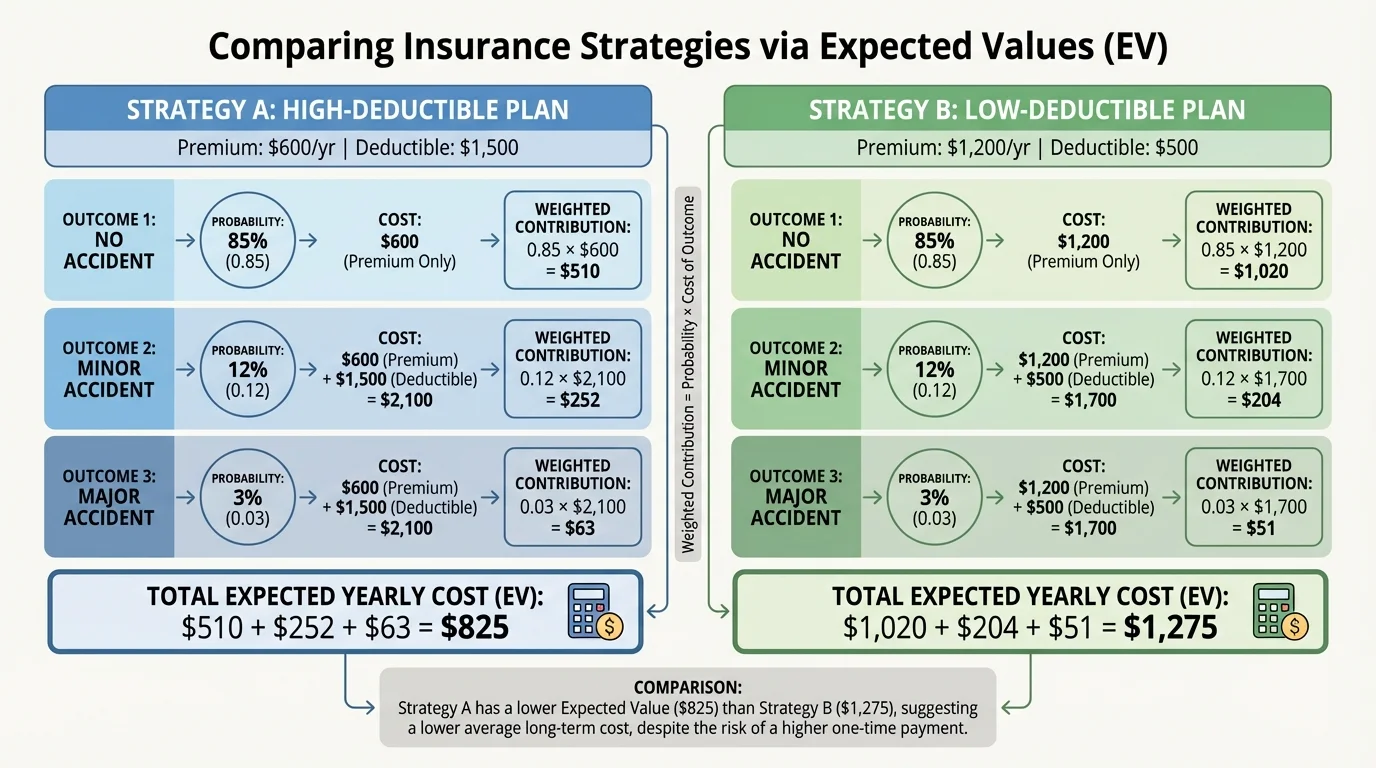
To evaluate a decision, we identify the possible outcomes, assign each one a probability, and assign each one a payoff or cost. As [Figure 1] shows, expected value combines these outcomes into one weighted average, where more likely outcomes affect the average more strongly than unlikely ones.
A payoff is the value connected to an outcome. In some settings a payoff is money gained. In others, especially insurance, it is easier to work with cost, meaning money paid. The expected value is found by multiplying each payoff by its probability and then adding the results:
\[E = \sum \big(\textrm{probability of outcome}\big)\big(\textrm{payoff of outcome}\big)\]
If there are three outcomes with probabilities \(p_1\), \(p_2\), and \(p_3\), and payoffs \(x_1\), \(x_2\), and \(x_3\), then
\[E = p_1x_1 + p_2x_2 + p_3x_3\]
For a cost problem, a lower expected value is better because you expect to spend less on average. For a profit problem, a higher expected value is better because you expect to gain more on average.
Expected value is the probability-weighted average of all possible outcomes.
Probability is the chance that an outcome occurs, written as a number from \(0\) to \(1\).
Payoff is the value associated with an outcome, such as money gained or money lost.
Expected value is especially useful when comparing several strategies that have different chances and different consequences. Insurance is a classic example because one option often has a lower premium and higher risk, while another has a higher premium and lower risk.
As [Figure 2] illustrates, suppose a driver is choosing between two automobile insurance policies. To compare them fairly, we need to include both the yearly premium and the amount the driver pays after an accident. A clear side-by-side model helps organize the decision into outcomes and costs instead of relying on guesswork.
Consider these two policies:
Policy H: high deductible, premium of $900 per year, deductible of $1,500.
Policy L: low deductible, premium of $1,300 per year, deductible of $500.
Now suppose there are three possible accident outcomes for the year:
Assume that for both accident types, the damage is large enough that the driver pays the full deductible. Then the driver's total yearly cost under each policy is:
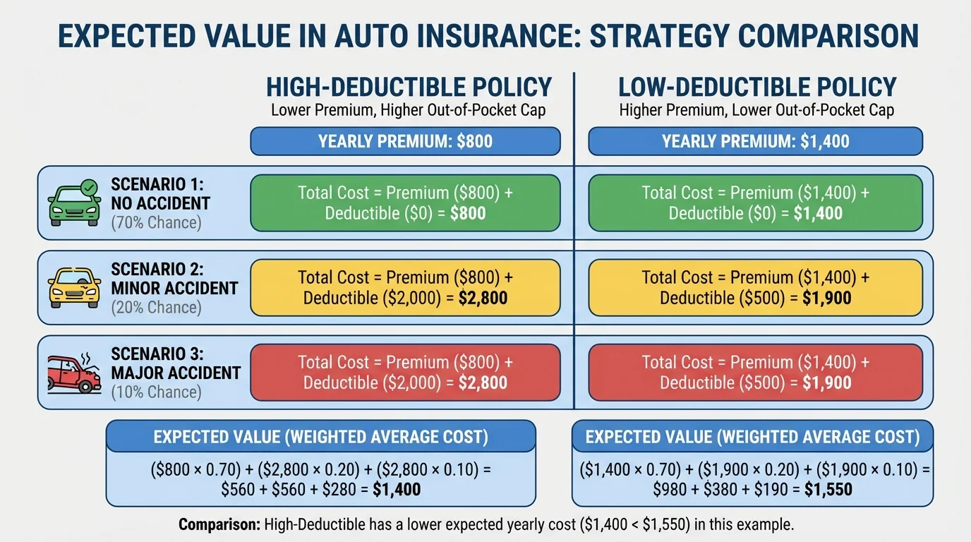
Notice something important: under this simplified model, both accident types lead to the same total cost within a policy because the deductible is the amount the driver pays. In more detailed models, a minor accident might cost less than the deductible, which changes the calculation. We will examine that kind of variation later.
Compare the expected yearly cost of the two insurance policies.
Step 1: Write the expected cost for Policy H.
Using the probabilities \(0.85\), \(0.12\), and \(0.03\):
\(E_H = 0.85(900) + 0.12(2400) + 0.03(2400)\)
Step 2: Calculate.
\(0.85(900) = 765\)
\(0.12(2400) = 288\)
\(0.03(2400) = 72\)
So \(E_H = 765 + 288 + 72 = 1{,}125\).
Step 3: Write the expected cost for Policy L.
\(E_L = 0.85(1300) + 0.12(1800) + 0.03(1800)\)
Step 4: Calculate.
\(0.85(1300) = 1105\)
\(0.12(1800) = 216\)
\(0.03(1800) = 54\)
So \(E_L = 1105 + 216 + 54 = 1{,}375\).
The expected yearly cost is $1,125 for Policy H and $1,375 for Policy L.
Conclusion: Based on expected value alone, the high-deductible policy is better in this scenario because it has the lower expected cost.
This result can feel counterintuitive. Some people expect the lower deductible to be the better financial deal because it protects more strongly after an accident. But if accidents are uncommon, paying a higher premium every year may cost more on average than taking the risk of a higher deductible.
Expected value depends completely on the probabilities and payoffs used in the model. If those values change, the better strategy can also change. That is why good decision-making requires reasonable assumptions. We should use probabilities that fit the situation: driving record, location, weather, traffic, age, and how much the car is used.
Suppose the driver has a higher accident risk:
Then the expected costs become:
For Policy H, \(E_H = 0.65(900) + 0.25(2400) + 0.10(2400) = 585 + 600 + 240 = 1{,}425\).
For Policy L, \(E_L = 0.65(1300) + 0.25(1800) + 0.10(1800) = 845 + 450 + 180 = 1{,}475\).
Policy H is still slightly better, but the gap has become much smaller. As the chance of accidents rises, the low-deductible policy starts looking more competitive.
Why the better choice can change
A deductible shifts part of the financial risk from the insurance company to the driver. A high deductible lowers the premium because the driver agrees to absorb more cost if an accident happens. A low deductible raises the premium because the insurer takes on more of that risk. Expected value measures which trade-off is better on average for a given set of accident probabilities.
This is one of the most important ideas in probability-based decisions: there is no universally best strategy. There is only the best strategy for a particular model.
Let us compare the same two policies for three different drivers. This helps show why one answer does not fit everyone.
| Driver profile | No accident | Minor accident | Major accident |
|---|---|---|---|
| Low-risk | \(0.92\) | \(0.07\) | \(0.01\) |
| Moderate-risk | \(0.80\) | \(0.16\) | \(0.04\) |
| High-risk | \(0.55\) | \(0.30\) | \(0.15\) |
Table 1. Probabilities of accident outcomes for three different driver profiles.
Compute and compare expected yearly costs.
Step 1: Low-risk driver.
Policy H: \(E_H = 0.92(900) + 0.07(2400) + 0.01(2400) = 828 + 168 + 24 = 1{,}020\)
Policy L: \(E_L = 0.92(1300) + 0.07(1800) + 0.01(1800) = 1196 + 126 + 18 = 1{,}340\)
Better choice: Policy H.
Step 2: Moderate-risk driver.
Policy H: \(E_H = 0.80(900) + 0.16(2400) + 0.04(2400) = 720 + 384 + 96 = 1{,}200\)
Policy L: \(E_L = 0.80(1300) + 0.16(1800) + 0.04(1800) = 1040 + 288 + 72 = 1{,}400\)
Better choice: Policy H.
Step 3: High-risk driver.
Policy H: \(E_H = 0.55(900) + 0.30(2400) + 0.15(2400) = 495 + 720 + 360 = 1{,}575\)
Policy L: \(E_L = 0.55(1300) + 0.30(1800) + 0.15(1800) = 715 + 540 + 270 = 1{,}525\)
Better choice: Policy L.
Conclusion: For low-risk and moderate-risk drivers, the high-deductible policy has the lower expected cost. For the high-risk driver, the low-deductible policy becomes better.
This is a realistic result. Drivers with higher accident risk are more likely to benefit from paying extra upfront to reduce out-of-pocket cost later.
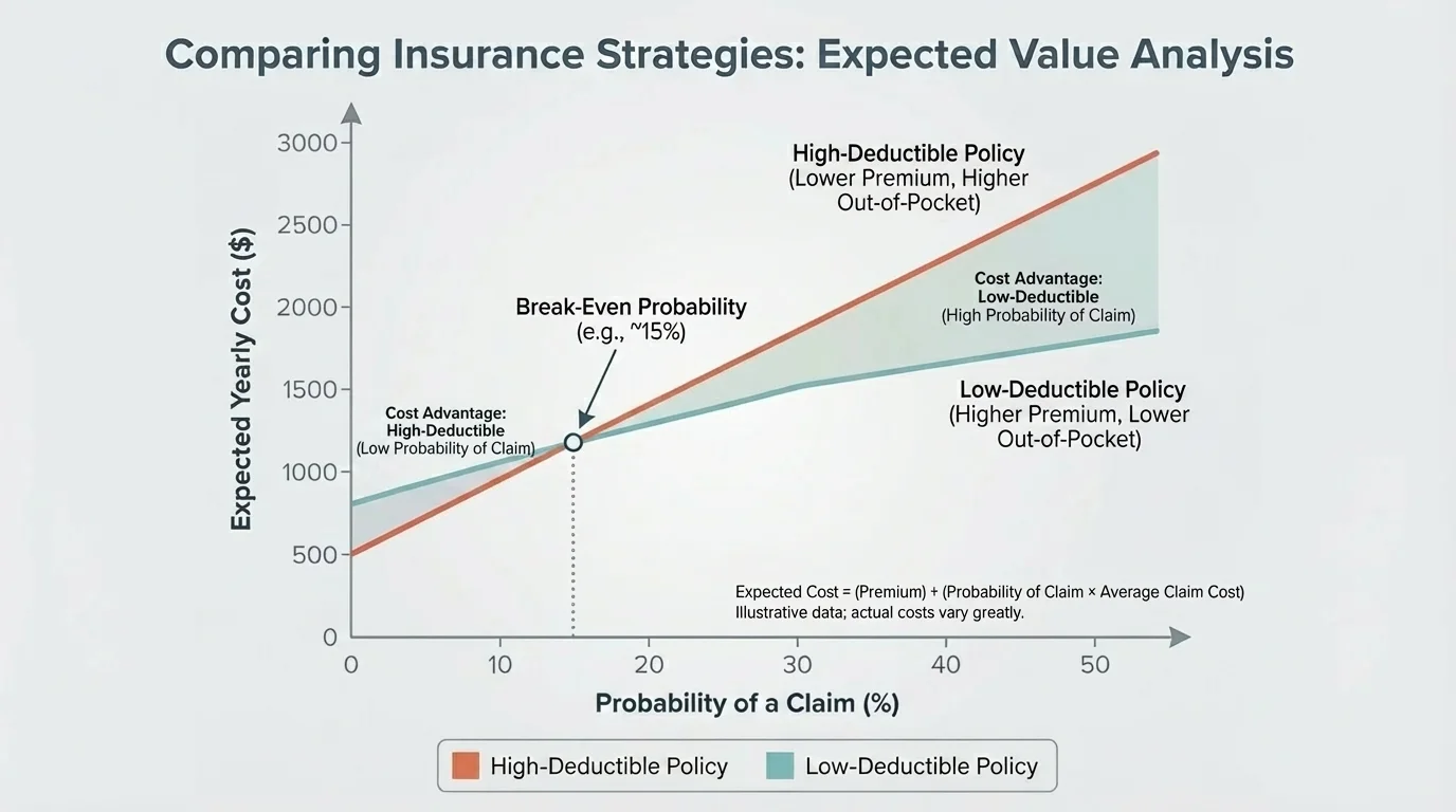
Sometimes we do not want to test many separate scenarios. Instead, we want to know the exact probability where two strategies become equally good. That point is called the break-even point. As [Figure 3] shows, it is the intersection where the expected-cost graphs of two strategies are equal.
Suppose we simplify the model into only two outcomes: no claim and a claim large enough to trigger the full deductible. Let \(p\) be the probability of having such a claim during the year.
Then the expected cost of Policy H is
\[E_H = 900 + 1500p\]
The expected cost of Policy L is
\[E_L = 1300 + 500p\]
Why do these formulas work? The premium is paid every year, so it is always included. The deductible is paid only if there is a claim, so it is multiplied by the probability \(p\).
Worked example 3: find the probability where the policies have the same expected cost.
Step 1: Set the expected costs equal.
\(900 + 1500p = 1300 + 500p\)
Step 2: Solve for \(p\).
Subtract \(500p\) from both sides: \(900 + 1000p = 1300\).
Subtract \(900\): \(1000p = 400\).
Divide by \(1000\): \(p = 0.4\).
Step 3: Interpret the result.
If the probability of a claim is \(0.4\), or \(40\%\), both policies have the same expected yearly cost.
So the break-even probability is \(0.4\).
If \(p < 0.4\), then Policy H has lower expected cost. If \(p > 0.4\), then Policy L has lower expected cost.
This threshold is powerful because it turns a complicated choice into one key question: is the chance of a claim above or below \(40\%\)? The visual comparison makes that shift easy to see because the lower-cost option changes at the intersection.
Break-even analysis is common in business as well. Companies compare machine options, advertising plans, and pricing strategies by finding when two cost models become equal.
Real insurance decisions are often more detailed than the simplified model above. A minor accident may cost less than the high deductible, meaning the driver pays the full repair cost rather than the deductible amount. That changes the expected value.
Suppose a minor accident costs $700 in repairs, while a major accident still exceeds either deductible. Use these probabilities: no accident \(0.80\), minor accident \(0.15\), major accident \(0.05\).
Then total yearly costs are:
Expected cost with different accident sizes
Step 1: Compute Policy H.
\(E_H = 0.80(900) + 0.15(1600) + 0.05(2400) = 720 + 240 + 120 = 1{,}080\)
Step 2: Compute Policy L.
\(E_L = 0.80(1300) + 0.15(1800) + 0.05(1800) = 1040 + 270 + 90 = 1{,}400\)
Conclusion: The high-deductible policy is still better by expected value in this case, and the difference is even larger because the minor accident cost is below the high deductible.
This example shows why the quality of the model matters. The better your outcomes match real life, the more useful your conclusion becomes.
Expected value is a strong mathematical tool, but it is not the whole story. Two strategies can have similar expected values while feeling very different in real life.
One important idea is risk tolerance. A driver might choose the low-deductible policy even if its expected cost is slightly higher because paying an extra $400 in premium is manageable, but paying a sudden $1,500 deductible would be difficult. In that case, the person is paying more on average for stability and protection against a large one-time cost.
Insurance companies rely heavily on expected value, but they also build in administrative costs, profit, and uncertainty. That is why insurance is usually a good deal for the company on average, even though it protects customers from rare but expensive losses.
Another issue is that expected value is a long-run average. A single year may not match the average at all. A driver may choose the policy with lower expected cost and still end up spending more that year because of bad luck. That does not mean the math was wrong; it means probability describes patterns over many repetitions, not guarantees for one event.
So when making a real decision, expected value should be combined with practical questions: Can I afford the deductible? How likely are these probabilities for me? How much uncertainty can I handle?
The same reasoning applies in many other settings. A store deciding whether to buy an extended warranty for equipment compares the probability of breakdown with the repair cost. A family deciding whether to buy phone protection compares the yearly fee with the chance and cost of damage. A sports coach choosing between a safe play and a risky play weighs each possible outcome by its probability and point value.
In medicine, doctors and patients sometimes compare treatment plans by expected benefits and expected side effects. In business, companies forecast profit by combining possible sales levels with their probabilities. In public policy, planners estimate expected losses from floods, fires, or storms when deciding how much protection to build.
"Good decisions are based on good models, not on guaranteed outcomes."
That idea is central to expected value. The goal is not to predict one exact future. The goal is to make the most reasonable decision using the information available now.
One mistake is forgetting to include all outcomes. If the listed probabilities do not add to \(1\), the model is incomplete. Another mistake is comparing only deductibles and forgetting premiums. The total yearly cost must include both.
A third mistake is using unrealistic probabilities. If a student assumes a \(50\%\) chance of a major accident for an ordinary driver, the result may be mathematically correct but not realistic. Expected value is only as trustworthy as the assumptions behind it.
A fourth mistake is misreading expected value as a promise. If the expected yearly cost is $1,125, that does not mean the driver will actually pay exactly $1,125. It means that over many similar years, the average cost would approach that amount.
Finally, do not confuse "lower expected cost" with "best for everyone." As we saw earlier in [Figure 2], the structure of premium and deductible creates different trade-offs, and those trade-offs matter differently for different drivers.