A company gives one worker a raise of \(\$2{,}000\) every year. Another worker's investment account grows at a percent growth rate of \(5\%\) each year. At first, both amounts may seem to be "going up steadily," but mathematically they are not the same kind of growth at all. One grows by adding the same amount again and again. The other grows by multiplying by the same factor again and again. That difference is one of the most important ideas in algebra because it tells us what kind of function models a situation accurately.
Many real situations can be misleading if you only look at whether something increases. A streaming service may add \(100\) users per day, while a social media trend may double every few days. Both are increasing, but one follows a straight-line pattern and the other follows a much more dramatic curve. Knowing whether a pattern has equal differences or equal factors helps you choose the right model, make better predictions, and avoid major errors.
In algebra, the two main models for these situations are linear functions and exponential functions. The key idea is not just how they look on a graph, but how their outputs behave when the inputs change by equal amounts.
Linear function: A function that can be written in the form \(f(x) = mx + b\), where \(m\) and \(b\) are constants. Its outputs change by equal differences over equal intervals of \(x\).
Exponential function: A function that can be written in the form \(f(x) = ab^x\), where \(a \neq 0\), \(b > 0\), and \(b \neq 1\). Its outputs change by equal factors over equal intervals of \(x\).
These two patterns are sometimes described as additive change and multiplicative change. Linear growth is additive: each equal step in \(x\) adds the same amount to the output. Exponential growth is multiplicative: each equal step in \(x\) multiplies the output by the same factor.
A linear function has the form \(f(x) = mx + b\). The number \(m\) is called the slope. If \(x\) increases by \(1\), then \(f(x)\) increases by \(m\). If \(x\) increases by \(2\), then \(f(x)\) increases by \(2m\). The change depends only on the interval length, not on where you start.
An exponential function has the form \(f(x) = ab^x\). The number \(b\) is the growth factor if \(b > 1\), or the decay factor if \(0 < b < 1\). If \(x\) increases by \(1\), then the output is multiplied by \(b\). If \(x\) increases by \(2\), then the output is multiplied by \(b^2\). Again, the behavior depends only on the interval length, not on the starting input.
Equal intervals means the input changes by the same amount each time, such as from \(x=1\) to \(x=3\) and from \(x=5\) to \(x=7\), where both intervals have length \(2\). For linear functions, outputs over those intervals differ by the same amount. For exponential functions, outputs over those intervals have the same ratio.
This gives us a powerful test. If a table shows constant first differences, the model is linear. If a table shows a constant ratio between successive outputs, the model is exponential. If neither pattern appears, the model is probably something else.
Let \(f(x) = mx + b\). To prove that equal intervals in \(x\) produce equal differences in output, compare the outputs at \(x\) and \(x+h\), where \(h\) is any fixed interval length.
Compute the difference:
\[\begin{aligned} f(x+h) - f(x) &= \big(m(x+h)+b\big) - (mx+b) \\&= mx + mh + b - mx - b \\&= mh\end{aligned}\]
The result is \(mh\). Notice what this means: the difference depends only on \(m\) and the interval length \(h\). It does not depend on the starting value \(x\). So whenever the input increases by the same amount \(h\), the output increases by the same amount \(mh\).
This is the formal proof of the statement that linear functions grow by equal differences over equal intervals. For example, if \(m=3\) and \(h=4\), then every interval of length \(4\) changes the output by \(3 \cdot 4 = 12\).
Subtracting outputs is how we measure a difference. If two intervals have the same length, then for a linear function the expression \(f(x+h)-f(x)\) is always the same.
This also works when the slope is negative. If \(m=-2\), then over every interval of length \(3\), the output changes by \((-2)(3)=-6\). The equal difference still exists; it is just a decrease instead of an increase.
Now let \(f(x) = ab^x\). To prove that equal intervals in \(x\) produce equal factors, compare \(f(x+h)\) with \(f(x)\) using a ratio rather than a difference.
Compute the ratio:
\[\begin{aligned} \frac{f(x+h)}{f(x)} &= \frac{ab^{x+h}}{ab^x} \\&= \frac{ab^x b^h}{ab^x} \\&= b^h\end{aligned}\]
The ratio is \(b^h\). Again, this depends only on the interval length \(h\), not on the starting input \(x\). So over every equal interval of length \(h\), the outputs are multiplied by the same factor \(b^h\).
This proves the exponential case. For instance, if \(b=2\) and \(h=3\), then every time \(x\) increases by \(3\), the output is multiplied by \(2^3=8\). If \(b=\dfrac{1}{2}\) and \(h=2\), then every interval of length \(2\) multiplies the output by \(\left(\dfrac{1}{2}\right)^2 = \dfrac{1}{4}\).
Why ratios matter for exponential functions: If you subtract outputs of an exponential function, the differences usually change from one interval to the next. But if you divide outputs over equal intervals, the ratio stays constant. That is the exponential signature.
This is why saying an exponential function "adds the same amount" is incorrect. Exponential change may start slowly, but because the multiplication repeats, the increases themselves become larger and larger when \(b > 1\).
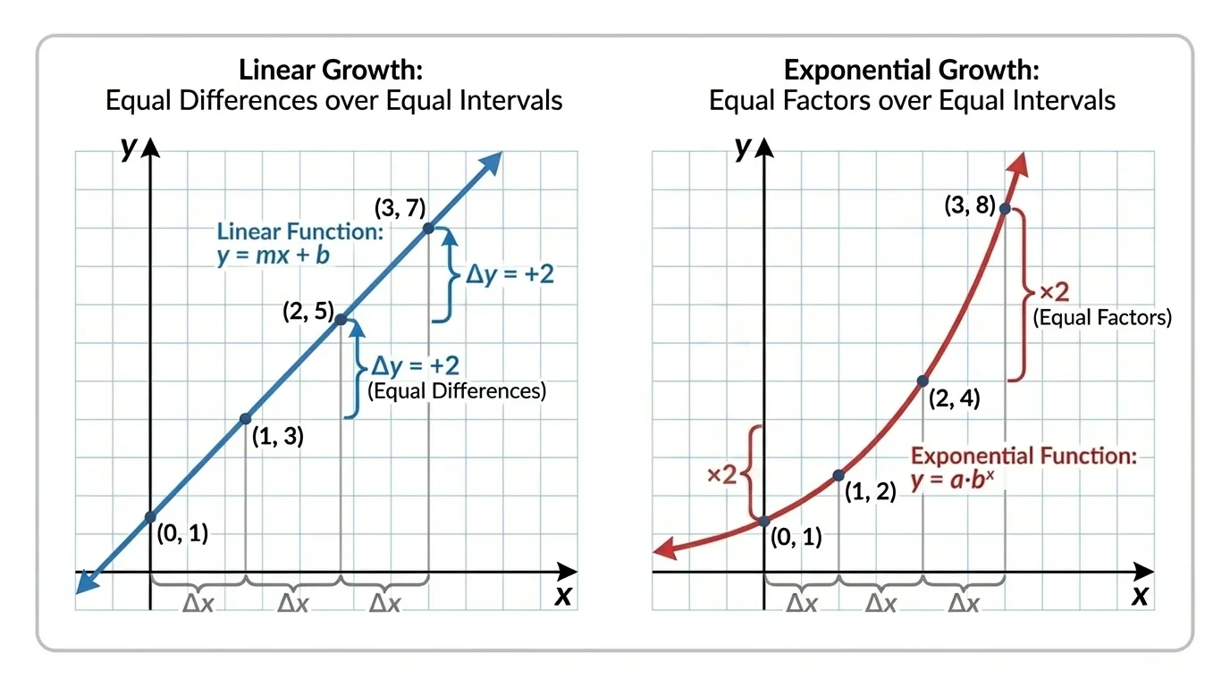
[Figure 1] Equal horizontal steps reveal the core pattern: a line rises by a constant vertical amount over equal intervals, while an exponential curve multiplies its output and becomes steeper. A graph gives a visual clue, but the proof comes from the algebraic expressions we already derived.
Consider these two functions: \(L(x)=2x+1\) and \(E(x)=3 \cdot 2^x\). If we list several values, the difference becomes obvious.
| \(x\) | \(L(x)=2x+1\) | Differences | \(E(x)=3\cdot 2^x\) | Ratios |
|---|---|---|---|---|
| \(0\) | \(1\) | \(3\) | ||
| \(1\) | \(3\) | \(+2\) | \(6\) | \(\times 2\) |
| \(2\) | \(5\) | \(+2\) | \(12\) | \(\times 2\) |
| \(3\) | \(7\) | \(+2\) | \(24\) | \(\times 2\) |
| \(4\) | \(9\) | \(+2\) | \(48\) | \(\times 2\) |
Table 1. A comparison of a linear function with constant differences and an exponential function with constant ratios.
For the linear model, the first differences are all \(+2\). For the exponential model, the ratio of each output to the one before it is always \(2\). These are not just numerical coincidences. They come directly from the forms \(mx+b\) and \(ab^x\).
On a graph, the linear function is a straight line because the rate of change is constant. The exponential function curves upward because each new increase is a multiple of what came before. This difference in shape matches the algebraic proofs and reinforces the pattern shown in [Figure 1].
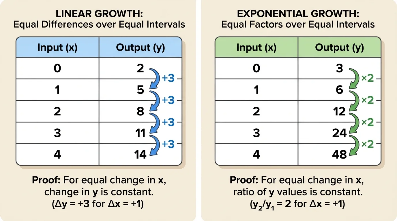
[Figure 2] Tables often reveal the pattern immediately, with one model changing by equal amounts and another changing by equal factors. But to classify a function confidently, you should connect the table pattern to the algebraic form.
We will work through several examples step by step.
Worked example 1
A function has values \((0,5)\), \((1,8)\), \((2,11)\), and \((3,14)\). Determine whether the function is linear or exponential.
Step 1: Look for equal differences.
The output changes are \(8-5=3\), \(11-8=3\), and \(14-11=3\).
Step 2: Interpret the pattern.
The differences are constant, so the function is linear.
Step 3: Write a model.
Since the slope is \(m=3\) and \(f(0)=5\), the rule is \(f(x)=3x+5\).
The function is linear because equal intervals of \(1\) produce equal differences of \(3\).
This example is typical of situations with a constant rate of change, such as earning the same hourly wage for each hour worked.
Worked example 2
A function has values \((0,4)\), \((1,12)\), \((2,36)\), and \((3,108)\). Determine whether the function is linear or exponential.
Step 1: Check the differences.
The differences are \(12-4=8\), \(36-12=24\), and \(108-36=72\). They are not constant.
Step 2: Check the ratios.
The ratios are \(\dfrac{12}{4}=3\), \(\dfrac{36}{12}=3\), and \(\dfrac{108}{36}=3\).
Step 3: Interpret the pattern.
The outputs are multiplied by \(3\) each time, so the function is exponential.
Step 4: Write a model.
Since \(f(0)=4\) and the growth factor is \(3\), the rule is \(f(x)=4\cdot 3^x\).
The function is exponential because equal intervals of \(1\) produce equal factors of \(3\).
This kind of pattern appears in repeated percentage growth, bacterial reproduction, and compound interest.
Worked example 3
Prove directly that the function \(g(x)=7-4x\) has equal differences over equal intervals of length \(h\).
Step 1: Write the expression for the output at \(x+h\).
\(g(x+h)=7-4(x+h)=7-4x-4h\).
Step 2: Subtract \(g(x)\).
\(g(x+h)-g(x)=(7-4x-4h)-(7-4x)=-4h\).
Step 3: Interpret the result.
The difference is always \(-4h\), which depends only on the interval length \(h\), not on \(x\).
So \(g(x)=7-4x\) is linear and changes by the same difference over every interval of length \(h\).
The negative sign means the function decreases, but it still has the linear property of constant difference.
Worked example 4
Prove directly that the function \(p(x)=6\left(\dfrac{1}{2}\right)^x\) has equal factors over equal intervals of length \(h\).
Step 1: Write the expression for the output at \(x+h\).
\(p(x+h)=6\left(\dfrac{1}{2}\right)^{x+h}\).
Step 2: Form the ratio.
\(\dfrac{p(x+h)}{p(x)}=\dfrac{6\left(\dfrac{1}{2}\right)^{x+h}}{6\left(\dfrac{1}{2}\right)^x}=\left(\dfrac{1}{2}\right)^h\).
Step 3: Interpret the result.
The ratio is always \(\left(\dfrac{1}{2}\right)^h\), which depends only on \(h\), not on \(x\).
So \(p(x)\) represents exponential decay and changes by the same factor over every interval of length \(h\).
Exponential decay is still exponential. The constant factor is just less than \(1\), so the outputs shrink rather than grow.
One common mistake is to think that "increasing" automatically means exponential. That is false. A function like \(y=100x+50\) increases, but it is linear because the difference is constant. Another common mistake is to think that exponential means "very fast." Exponential functions can grow slowly at first or decay instead of grow. What matters is the repeated multiplication, not how dramatic the graph looks at the beginning.
A second important point is that not every non-linear pattern is exponential. Consider the quadratic function \(q(x)=x^2\). Its outputs for \(x=0,1,2,3,4\) are \(0,1,4,9,16\). The differences are \(1,3,5,7\), which are not constant, and the ratios are not constant either. So quadratic functions fit neither the linear signature nor the exponential signature.
A quantity that doubles every day can stay small for a while and then suddenly become enormous. That surprise comes from repeated multiplication, which is why exponential growth often feels deceptive at first.
Also remember that equal intervals do not have to be intervals of length \(1\). For a linear function, every interval of length \(5\) produces the same difference. For an exponential function, every interval of length \(5\) produces the same factor. The interval length can be any constant \(h\).
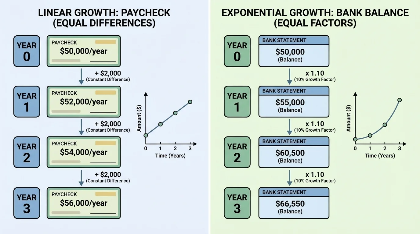
A fixed yearly raise and a percentage-based increase are not the same. If your salary increases by \(\$2{,}000\) each year, the pattern is linear because the same amount is added each year.
If an investment grows by \(4\%\) each year, the pattern is exponential because each year multiplies the balance by \(1.04\).
[Figure 3] Suppose a car loses \(\$1{,}500\) in value each year. That is approximately linear depreciation, modeled by subtracting the same amount over equal intervals. But if a medicine in the bloodstream loses half its amount every hour, the pattern is exponential decay because each hour multiplies the amount by \(\dfrac{1}{2}\).
Population models also highlight the difference. If a town adds about \(800\) residents every year, a linear model may work well over a short period. If a bacterial population triples every \(6\) hours, an exponential model is much more accurate because the number added in each interval depends on how many bacteria are already present.
Technology gives another example. If a phone plan charges a base fee plus a fixed amount per gigabyte, the total cost is linear in the amount of data used. If a video goes viral and the number of shares multiplies by about \(1.8\) every hour, the spread is exponential. The difference between adding and multiplying is exactly what separates these models.
The deeper idea is that linear and exponential functions respond differently to equal changes in input. For a linear function, the meaningful comparison is subtraction:
\[f(x+h)-f(x)=mh\]
For an exponential function, the meaningful comparison is division:
\[\frac{f(x+h)}{f(x)}=b^h\]
These two expressions capture the heart of the topic. If equal intervals give equal differences, the model is linear. If equal intervals give equal factors, the model is exponential. That distinction helps you read tables, interpret graphs, build formulas, and model the real world with much greater accuracy.