When you ride in a car at a steady speed, something interesting happens: as time increases, distance increases too. If you travel for twice as long, you go twice as far. That kind of pattern appears everywhere—in money spent, pages read, water poured, and miles biked. Mathematics gives us a powerful way to describe these changing quantities by using variables, equations, tables, and graphs.
Sometimes one amount changes because another amount changes. Suppose a runner keeps the same pace. The longer the runner moves, the farther the runner travels. These are two quantities that change in relationship to one another.
When we use letters to stand for numbers, those letters are called variables. A variable can represent a quantity that may change. In a travel problem, we might use \(t\) for time and \(d\) for distance.
In many real-world problems, one quantity is chosen first. Then the other quantity is determined from it. If you know the number of hours a car travels, you can find the distance. If you know the number of tickets bought, you can find the total cost. This is why learning how quantities depend on each other is so useful.
Independent variable is the quantity you choose or control first.
Dependent variable is the quantity that changes because of the independent variable.
An equation shows the rule connecting the two variables.
Ordered pairs are pairs of numbers written like \((x, y)\), used to show matching input and output values on a graph.
Think of a vending machine. You choose how many drinks to buy. The total cost depends on that choice. The number of drinks is the independent variable, and the total cost is the dependent variable.
It helps to think of the independent variable as the input and the dependent variable as the output. For example, if each notebook costs $3, then the number of notebooks is the input, and the total cost is the output.
If \(n\) stands for the number of notebooks, and \(c\) stands for the total cost, the relationship is
\(c = 3n\)
This equation says the cost depends on the number of notebooks. If \(n = 4\), then \(c = 12\). If \(n = 7\), then \(c = 21\).
Remember that a variable is just a symbol for a number. Also remember that when one variable is written alone on one side of an equation, it often means we are showing how that variable is found from the other variable.
Many relationships in grade 6 involve a constant rate. That means every time the independent variable goes up by the same amount, the dependent variable also goes up by the same amount. In \(c = 3n\), every increase of \(1\) notebook adds $3 to the cost.
To write an equation, first decide what the two quantities are. Next, decide which one depends on the other. Then look for the rule connecting them.
Suppose a car travels at a constant speed of \(65\) miles per hour. Let \(t\) be the time in hours and \(d\) be the distance in miles. Since distance depends on time, the equation is
\(d = 65t\)
This means that after \(1\) hour, the car goes \(65\) miles. After \(2\) hours, it goes \(130\) miles. After \(3\) hours, it goes \(195\) miles.
Notice how the variable names matter. Writing \(d = 65t\) tells us clearly that distance depends on time. Writing \(t = 65d\) would not make sense in this situation.
How to identify the dependent variable
Ask yourself, "If I know one quantity first, which other quantity can I calculate from it?" In a motion problem, once you know time, you can calculate distance. In a shopping problem, once you know the number of items, you can calculate cost. The calculated quantity is the dependent variable.
Some relationships include a starting amount. For example, if a bike rental shop charges $8 to rent a bike plus $5 for each hour, the total cost is not just based on hours. It includes a beginning fee.
If \(h\) is the number of hours and \(c\) is the cost, then
\(c = 5h + 8\)
Now the dependent variable still depends on the independent variable, but there is also a fixed starting value.
A table is one of the clearest ways to organize matching values. You choose values for the independent variable and use the equation to find the dependent variable.
For the equation \(d = 65t\), we can make a table of times and distances.
| Time \((t)\) in hours | Distance \((d)\) in miles |
|---|---|
| \(0\) | \(0\) |
| \(1\) | \(65\) |
| \(2\) | \(130\) |
| \(3\) | \(195\) |
| \(4\) | \(260\) |
Table 1. Values showing the relationship between time and distance for \(d = 65t\).
Each row in the table gives an ordered pair: \((0,0)\), \((1,65)\), \((2,130)\), \((3,195)\), and \((4,260)\). The first number is the independent variable, and the second number is the dependent variable.
Tables help us notice patterns. In this table, whenever time increases by \(1\), distance increases by \(65\). That repeating change tells us the relationship has a constant rate.
Airplanes, cars, and even moving walkways can all be modeled with equations when their speeds stay constant. The same idea helps scientists, athletes, and engineers predict what will happen next.
You can also work backward from a table. If you notice that every output is \(4\) times the input, then the equation is \(y = 4x\). If every output is \(4\) times the input plus \(2\), then the equation is \(y = 4x + 2\).
A graph helps us see a relationship quickly, as [Figure 1] illustrates with time and distance on a coordinate plane. A graph shows how the dependent variable changes as the independent variable changes.
On a graph, the independent variable is usually placed on the horizontal axis, also called the \(x\)-axis. The dependent variable is usually placed on the vertical axis, also called the \(y\)-axis. For \(d = 65t\), time goes on the horizontal axis and distance goes on the vertical axis.
Using the table above, we plot the ordered pairs \((0,0)\), \((1,65)\), \((2,130)\), \((3,195)\), and \((4,260)\). Because the speed is constant, the points lie on a straight line.
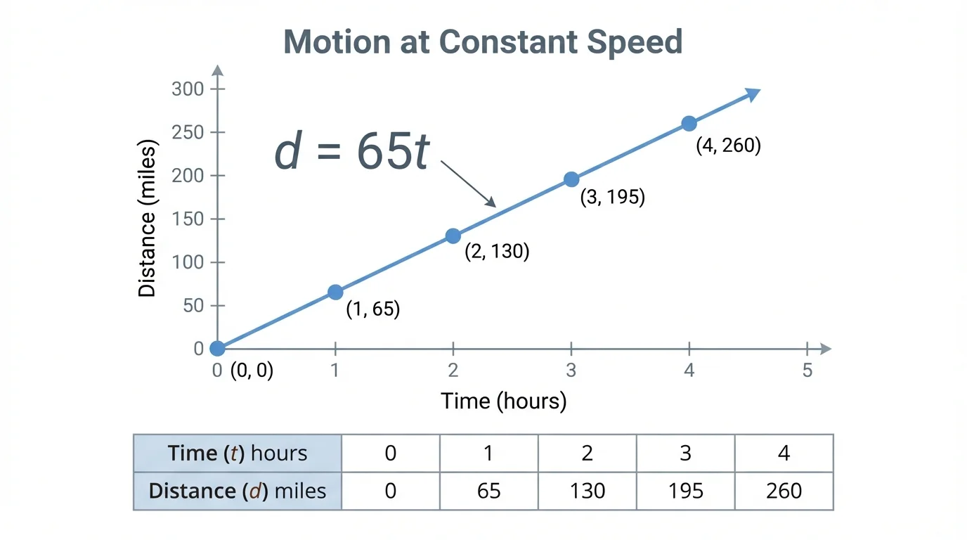
A straight line on the graph means the relationship changes at a constant rate. The steeper the line, the faster the distance increases for each hour.
The graph, table, and equation all describe the same situation. The equation gives the rule, the table gives selected values, and the graph gives a picture of the pattern. Later, when we compare representations again, [Figure 1] still helps us see why constant speed creates a straight-line graph.
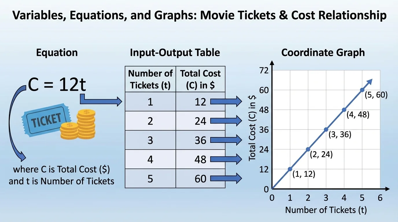
Let's solve several examples step by step. As you work through them, watch how the equation, the table, and the graph all connect. In some cases, the relationship can be viewed in a table and on a graph, as [Figure 2] shows for a cost situation.
Worked Example 1: Distance and time at constant speed
A train travels at \(50\) miles per hour. Write an equation for distance \(d\) in terms of time \(t\), and find the distance after \(3\) hours.
Step 1: Identify the quantities.
Time \(t\) is the independent variable, and distance \(d\) is the dependent variable.
Step 2: Write the rule.
At \(50\) miles per hour, distance equals speed times time, so \(d = 50t\).
Step 3: Substitute \(t = 3\).
\(d = 50(3) = 150\).
The equation is \(d = 50t\) and after \(3\) hours the train travels \(150\) miles.
Notice that this equation has no starting amount. When \(t = 0\), the distance is \(0\). That means the graph starts at the origin.
Worked Example 2: Total ticket cost
A movie ticket costs $9. Let \(n\) be the number of tickets and \(c\) be the total cost. Write an equation and make a few ordered pairs.
Step 1: Decide which quantity depends on the other.
The total cost depends on how many tickets are bought, so \(n\) is independent and \(c\) is dependent.
Step 2: Write the equation.
Each ticket adds $9, so \(c = 9n\).
Step 3: Find ordered pairs.
If \(n = 1\), then \(c = 9\), giving \((1,9)\).
If \(n = 2\), then \(c = 18\), giving \((2,18)\).
If \(n = 3\), then \(c = 27\), giving \((3,27)\).
The relationship is \(c = 9n\) with ordered pairs such as \((1,9)\), \((2,18)\), and \((3,27)\).
In this example, the output grows by the same amount each time. Each extra ticket adds $9, so the graph forms a straight pattern just like a constant-speed graph.
Worked Example 3: Pages read over time
Lena reads \(12\) pages every hour. Let \(h\) be the number of hours and \(p\) be the number of pages read. Write an equation, then find the number of pages after \(5\) hours.
Step 1: Identify the variables.
Hours \(h\) are the independent variable. Pages \(p\) are the dependent variable.
Step 2: Write the equation.
Because Lena reads \(12\) pages each hour, \(p = 12h\).
Step 3: Substitute \(h = 5\).
\(p = 12(5) = 60\).
The equation is \(p = 12h\) and after \(5\) hours Lena reads \(60\) pages.
This kind of equation can describe many everyday situations: miles traveled, songs downloaded, bottles packed, or dollars earned per hour.
Worked Example 4: A relationship with a starting value
A gym charges a one-day fee of $15 plus $4 for each hour of rock climbing. Let \(h\) be the hours and \(c\) be the total cost.
Step 1: Find the fixed amount and the rate.
The fixed amount is $15, and the rate is $4 per hour.
Step 2: Write the equation.
\(c = 4h + 15\).
Step 3: Find the cost for \(3\) hours.
\(c = 4(3) + 15 = 12 + 15 = 27\).
The equation is \(c = 4h + 15\) and the cost for \(3\) hours is $27.
This graph is still a straight line, but it does not start at \((0,0)\). Instead, when \(h = 0\), the cost is \(15\). That starting point matters.
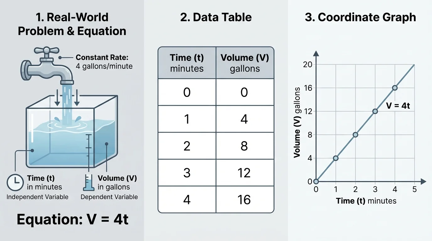
One relationship can be represented in three connected ways, as [Figure 3] shows with an equation, a value table, and a graph for the same situation. Learning to move between these forms is an important algebra skill.
Suppose a container fills with \(3\) gallons of water each minute. Let \(m\) be the number of minutes and \(g\) be the gallons of water. The equation is \(g = 3m\). From that equation, we can make a table. From the table, we can plot points on a graph.
| Minutes \((m)\) | Gallons \((g)\) |
|---|---|
| \(0\) | \(0\) |
| \(1\) | \(3\) |
| \(2\) | \(6\) |
| \(3\) | \(9\) |
| \(4\) | \(12\) |
Table 2. Matching values for the water-filling equation \(g = 3m\).
If someone gives you the graph first, you can read points and build a table. If someone gives you the table first, you can look for a pattern and write an equation. If someone gives you the equation first, you can generate as many ordered pairs as needed.
For the water example, each increase of \(1\) minute adds \(3\) gallons. That same pattern appears in the table, in the equation coefficient, and in the steepness of the line on the graph. This is why [Figure 3] is so useful: it displays the same relationship in three forms.
These ideas are not only for math class. They are used in science, business, sports, and technology. A coach might compare running time and distance. A delivery company might compare the number of packages and total weight. A streaming service might compare months subscribed and total cost.
Here are a few examples of real-world relationships:
In each case, one quantity depends on another. The equation provides a rule, the table organizes values, and the graph helps show the pattern visually.
"A graph is a picture of a pattern."
— An important algebra idea
Even when the numbers get larger, the thinking stays the same: identify the variables, decide which depends on the other, write an equation, and use a table or graph to understand the relationship.
One common mistake is switching the variables. If cost depends on number of items, then the cost variable should be alone on one side of the equation, like \(c = 5n\), not \(n = 5c\).
Another mistake is placing the variables on the wrong axes. The independent variable usually belongs on the horizontal axis, and the dependent variable usually belongs on the vertical axis.
A third mistake is writing ordered pairs in the wrong order. If time is independent and distance is dependent, then after \(2\) hours and \(130\) miles, the ordered pair is \((2,130)\), not \((130,2)\).
What a constant rate looks like
When equal changes in the independent variable cause equal changes in the dependent variable, the relationship has a constant rate. In many grade-level situations, this creates a straight-line graph. The number multiplying the independent variable in the equation tells the rate.
Checking your work in all three forms can help you catch mistakes. If the table values do not match the equation, or the graph points do not match the table, something needs to be fixed.
Suppose an equation is \(y = 7x\). If \(x\) increases by \(1\), then \(y\) increases by \(7\). If \(x\) increases by \(2\), then \(y\) increases by \(14\). This predictable pattern tells us a lot about the relationship.
If the equation is \(y = 7x + 4\), then the change is still \(7\) for every increase of \(1\) in \(x\), but now there is also a starting value of \(4\). That means when \(x = 0\), \(y = 4\).
Understanding these patterns helps you compare different situations. A car traveling at \(65\) miles per hour changes faster than a bike traveling at \(12\) miles per hour because the coefficient of the time variable is larger. On a graph, that means the car's line is steeper than the bike's line, just as we saw earlier in [Figure 1].
When you can move easily between words, equations, tables, and graphs, you are doing real algebra. You are showing not just numbers, but how quantities are connected.