What do image filters on your phone, statistics in sports, and 3D graphics in movies all have in common? They rely heavily on matrices—rectangular arrays of numbers that package data and operations in a compact, powerful way.
Whenever a computer works with data that naturally forms a grid—like pixels in an image, scores of players across multiple games, or connection strengths in a social network—it often represents that data as a matrix. Operations on this data, such as combining statistics, scaling intensities, or transforming 3D coordinates, are done using matrix addition, subtraction, and multiplication.
Learning how to add, subtract, and multiply matrices is not just an abstract algebra skill. It is a core tool for modern applications in engineering, computer science, physics, and data science.
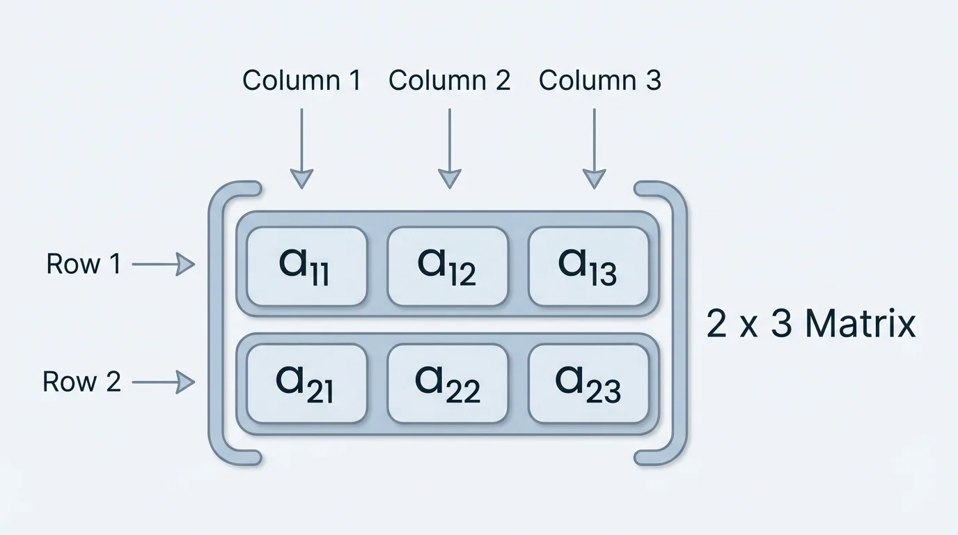
A matrix is a rectangular array of numbers arranged in rows and columns. For example, a matrix with 2 rows and 3 columns might look like this:
\[A = \begin{bmatrix} 1 & 4 & -2 \\ 0 & 5 & 3 \end{bmatrix}\]
We say that matrix \(A\) is a \(2 \times 3\) matrix ("2 by 3"): it has 2 rows and 3 columns. The entry in row \(i\), column \(j\) is often written as \(a_{ij}\). For example, in the matrix above, \(a_{12} = 4\) because it is in the first row, second column.
The idea of rows and columns, and how they form the dimensions of a matrix, is at the heart of which operations are allowed, as shown in [Figure 1]. When we talk about whether we can add or multiply two matrices, the first thing we check is their sizes.
Key terms
We often use capital letters like \(A, B, C\) for matrices and lowercase letters with subscripts like \(a_{ij}\) for their entries.
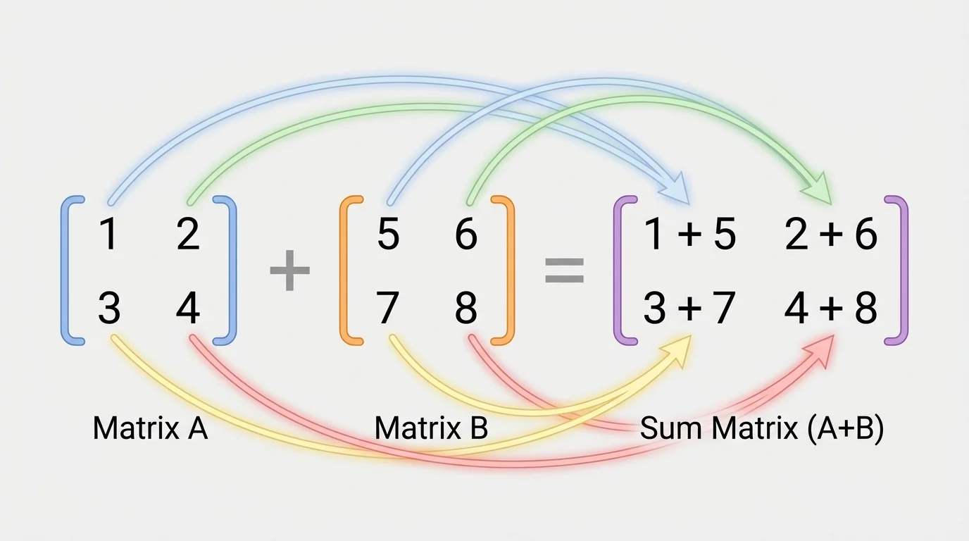
Matrix addition and subtraction are the simplest operations. They work entry by entry. However, there is a crucial rule: to add or subtract two matrices, they must have the same dimensions, as illustrated in [Figure 2].
Suppose \(A\) and \(B\) are both \(m \times n\) matrices. Their sum \(C = A + B\) is another \(m \times n\) matrix where each entry is
\[c_{ij} = a_{ij} + b_{ij}.\]
This means we add the numbers in the same position in each matrix.
For subtraction \(C = A - B\), we use
\[c_{ij} = a_{ij} - b_{ij}.\]
If the matrices do not have the same size, \(A + B\) and \(A - B\) are not defined.
Example 1: Adding and subtracting matrices
Let
\[A = \begin{bmatrix} 2 & -1 \\ 3 & 4 \end{bmatrix}, \quad B = \begin{bmatrix} 5 & 0 \\ -2 & 7 \end{bmatrix}.\]
Step 1: Add the matrices.
Add entry by entry:
\[A + B = \begin{bmatrix} 2 + 5 & -1 + 0 \\ 3 + (-2) & 4 + 7 \end{bmatrix} = \begin{bmatrix} 7 & -1 \\ 1 & 11 \end{bmatrix}.\]
Step 2: Subtract the matrices.
\[A - B = \begin{bmatrix} 2 - 5 & -1 - 0 \\ 3 - (-2) & 4 - 7 \end{bmatrix} = \begin{bmatrix} -3 & -1 \\ 5 & -3 \end{bmatrix}.\]
Both operations are valid because \(A\) and \(B\) are both \(2 \times 2\) matrices.
As [Figure 2] suggests, you can think of addition as stacking two grids of numbers and combining them cell by cell.
Before learning full matrix multiplication, we look at a simpler operation: multiplying a matrix by a scalar, which is just a regular real number.
If \(k\) is a real number and \(A\) is a matrix, then \(kA\) is the matrix you get by multiplying every entry of \(A\) by \(k\). If \(A\) is \(m \times n\), then \(kA\) is also \(m \times n\).
Formally, if \(A = [a_{ij}]\), then
\[(kA)_{ij} = k \cdot a_{ij}.\]
Example 2: Scalar multiplication
Let
\[A = \begin{bmatrix} 1 & -3 & 4 \\ 0 & 2 & -5 \end{bmatrix}, \quad k = -2.\]
Step 1: Multiply each entry by \(-2\).
\[-2A = \begin{bmatrix} -2 \cdot 1 & -2 \cdot (-3) & -2 \cdot 4 \\ -2 \cdot 0 & -2 \cdot 2 & -2 \cdot (-5) \end{bmatrix} = \begin{bmatrix} -2 & 6 & -8 \\ 0 & -4 & 10 \end{bmatrix}.\]
This operation stretches or flips the matrix entries, similar to how multiplying a vector by a scalar stretches its length.
Matrix multiplication is more subtle than scalar multiplication. It does not work entry by entry. Instead, it combines rows of the first matrix with columns of the second.
First, we must know when the product is defined, as emphasized in [Figure 3]. Suppose matrix \(A\) is \(m \times n\) and matrix \(B\) is \(n \times p\). Then the product \(AB\) is defined, and it will be an \(m \times p\) matrix.
We often state the dimension rule like this: for \(A\) of size \(m \times n\) and \(B\) of size \(n \times p\), the product \(AB\) has size \(m \times p\). The inner dimensions \(n\) and \(n\) must match, and the outer dimensions \(m\) and \(p\) give the size of the result.
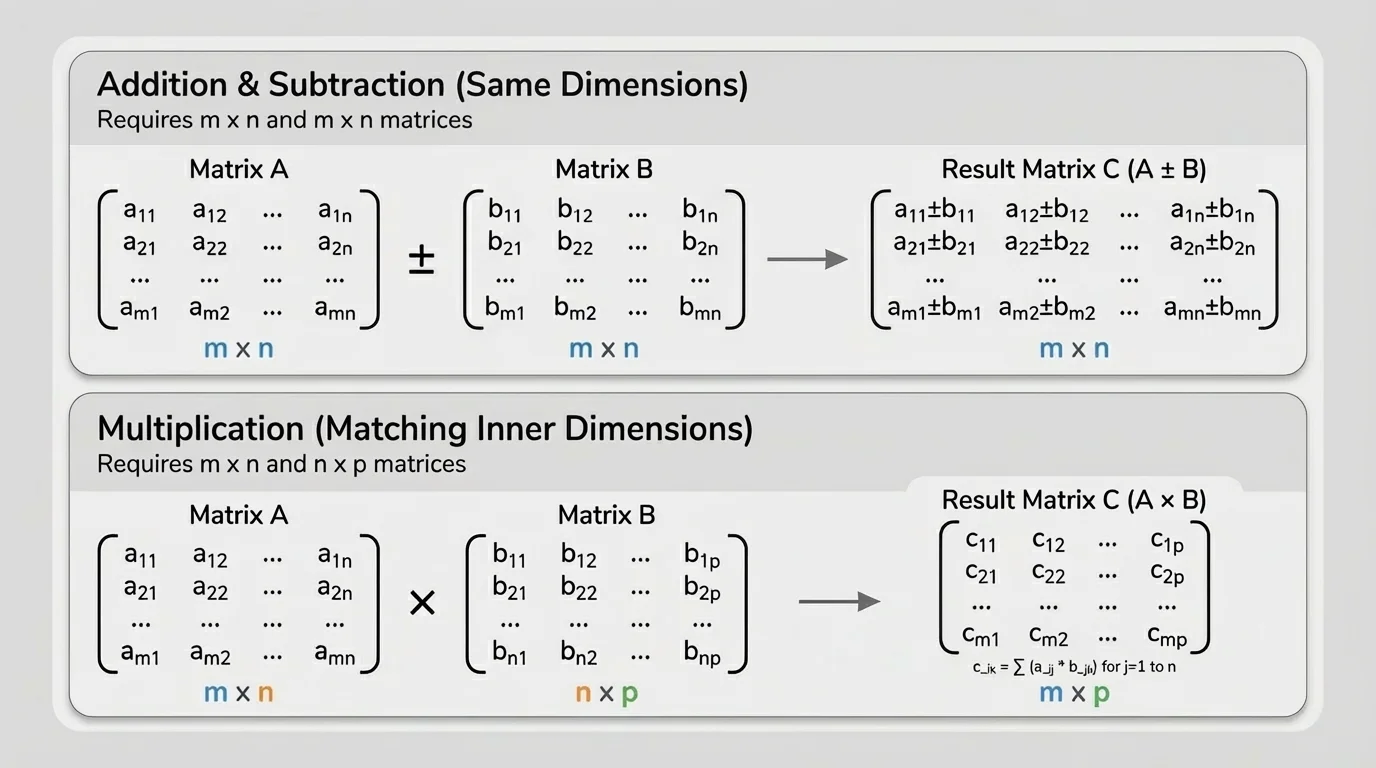
If the number of columns of \(A\) does not equal the number of rows of \(B\), then \(AB\) is not defined.
Also, note an important fact: in general, \(AB \neq BA\), and sometimes \(BA\) is not even defined. Matrix multiplication is usually not commutative.
When the product \(AB\) is defined, we use the row-by-column rule: each entry of the product is a dot product of a row of \(A\) with a column of \(B\).
Suppose \(A\) is \(m \times n\) and \(B\) is \(n \times p\). Let the product be \(C = AB\), an \(m \times p\) matrix, as shown in [Figure 4]. To find entry \(c_{ij}\) (row \(i\), column \(j\)), we:
Formally,
\[c_{ij} = a_{i1}b_{1j} + a_{i2}b_{2j} + \cdots + a_{in}b_{nj}.\]
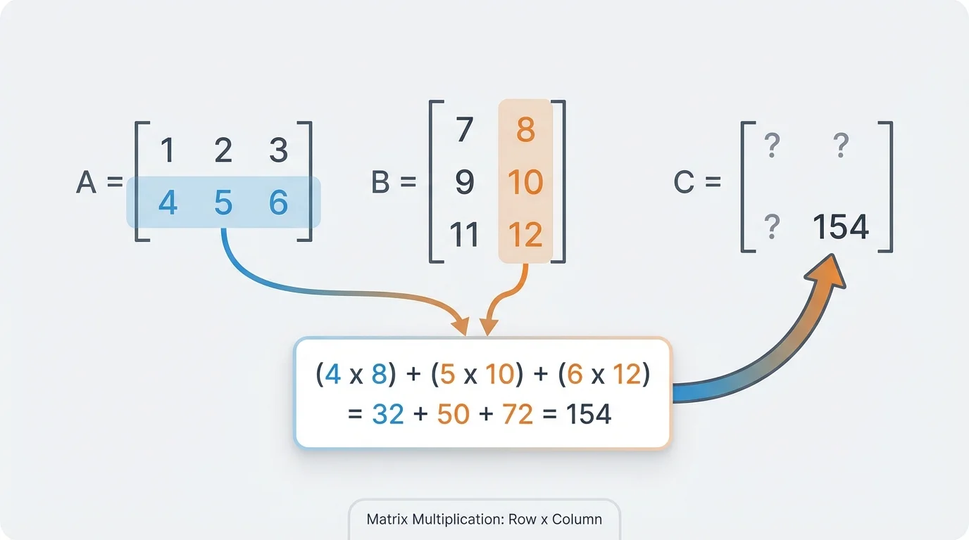
So each entry of the product is one dot product. As [Figure 4] illustrates, you repeat this for every row of \(A\) and every column of \(B\).
Example 3: Multiplying a \(2 \times 3\) matrix by a \(3 \times 2\) matrix
Let
\[A = \begin{bmatrix} 1 & 2 & 3 \\ 4 & 5 & 6 \end{bmatrix}, \quad B = \begin{bmatrix} 7 & 8 \\ 9 & 10 \\ 11 & 12 \end{bmatrix}.\]
Step 1: Check dimensions.
Matrix \(A\) is \(2 \times 3\), matrix \(B\) is \(3 \times 2\). The inner dimensions (3 and 3) match, so \(AB\) is defined and will be \(2 \times 2\).
Step 2: Compute \(c_{11}\) (row 1, column 1).
Row 1 of \(A\) is \([1, 2, 3]\), column 1 of \(B\) is \([7, 9, 11]^T\).
\[c_{11} = 1\cdot 7 + 2\cdot 9 + 3\cdot 11 = 7 + 18 + 33 = 58.\]
Step 3: Compute \(c_{12}\) (row 1, column 2).
Row 1 of \(A\) is \([1, 2, 3]\), column 2 of \(B\) is \([8, 10, 12]^T\).
\[c_{12} = 1\cdot 8 + 2\cdot 10 + 3\cdot 12 = 8 + 20 + 36 = 64.\]
Step 4: Compute \(c_{21}\) (row 2, column 1).
Row 2 of \(A\) is \([4, 5, 6]\), column 1 of \(B\) is \([7, 9, 11]^T\).
\[c_{21} = 4\cdot 7 + 5\cdot 9 + 6\cdot 11 = 28 + 45 + 66 = 139.\]
Step 5: Compute \(c_{22}\) (row 2, column 2).
Row 2 of \(A\) is \([4, 5, 6]\), column 2 of \(B\) is \([8, 10, 12]^T\).
\[c_{22} = 4\cdot 8 + 5\cdot 10 + 6\cdot 12 = 32 + 50 + 72 = 154.\]
So the product is
\[AB = \begin{bmatrix} 58 & 64 \\ 139 & 154 \end{bmatrix}.\]
A special and very important case (used in many applications) is multiplying a matrix by a column vector. If \(A\) is \(m \times n\) and \(\mathbf{x}\) is an \(n \times 1\) column vector, then \(A\mathbf{x}\) is an \(m \times 1\) column vector. It is computed by taking dot products of rows of \(A\) with the vector \(\mathbf{x}\).
Matrix operations share many properties with real-number arithmetic, but not all.
| Operation | Property | Statement |
|---|---|---|
| Addition | Commutative | If \(A\) and \(B\) have the same size, then \(A + B = B + A\). |
| Addition | Associative | \(A + (B + C) = (A + B) + C\) when all three have the same size. |
| Scalar mult. | Distributive | \(k(A + B) = kA + kB\). |
| Matrix mult. | Associative | If dimensions match, \((AB)C = A(BC)\). |
| Matrix mult. | Left distributive | \(A(B + C) = AB + AC\). |
| Matrix mult. | Right distributive | \((A + B)C = AC + BC\). |
| Matrix mult. | Not commutative | In general, \(AB \neq BA\), even when both products are defined. |
Table 1. Selected properties of matrix operations.
There are also special matrices that behave like numbers 0 and 1:
Matrix operations are deeply connected to real-world problems 🌍. Here are some key areas:
1. Systems of linear equations. A system like
\[\begin{cases} 2x + 3y = 5 \\ -x + 4y = 1 \end{cases}\]
can be written as a matrix equation
\[A\mathbf{x} = \mathbf{b}, \quad \textrm{where } A = \begin{bmatrix} 2 & 3 \\ -1 & 4 \end{bmatrix}, \ \mathbf{x} = \begin{bmatrix} x \\ y \end{bmatrix}, \ \mathbf{b} = \begin{bmatrix} 5 \\ 1 \end{bmatrix}.\]
Solving the system becomes understanding how multiplication by \(A\) transforms the vector \(\mathbf{x}\).
2. Computer graphics and transformations. In 2D and 3D graphics, points are represented as vectors, and transformations such as rotations, reflections, and scaling are represented as matrices. Multiplying a transformation matrix by a coordinate vector gives a new coordinate vector. Composing several transformations corresponds to multiplying matrices.
3. Data analysis and statistics. Large datasets (for example, exam scores of many students across many tests) are stored as matrices. Combining datasets, computing weighted sums, or changing the scale of scores uses matrix addition, subtraction, and scalar multiplication. More advanced tools (like principal component analysis) rely heavily on matrix multiplication.
4. Networks and graphs. Social networks, communication networks, and transportation systems can be described using adjacency matrices, where entry \(a_{ij}\) might represent a connection from node \(i\) to node \(j\). Powers of the adjacency matrix (repeated multiplication) encode information about paths of length 2, 3, and so on.
Example 4: Checking when operations are defined
Suppose
\[A \textrm{ is } 2 \times 3, \quad B \textrm{ is } 2 \times 3, \quad C \textrm{ is } 3 \times 2.\]
Step 1: Is \(A + B\) defined?
Yes. Both are \(2 \times 3\), so \(A + B\) is \(2 \times 3\).
Step 2: Is \(A + C\) defined?
No. \(A\) is \(2 \times 3\) and \(C\) is \(3 \times 2\); they do not have the same dimensions.
Step 3: Is \(AC\) defined?
Yes. \(A\) is \(2 \times 3\) and \(C\) is \(3 \times 2\). The inner dimensions (3 and 3) match, so \(AC\) is \(2 \times 2\).
Step 4: Is \(CA\) defined?
Yes. \(C\) is \(3 \times 2\) and \(A\) is \(2 \times 3\). The inner dimensions (2 and 2) match, so \(CA\) is \(3 \times 3\).
This example highlights how the order matters for multiplication and how dimension checks control what is possible.
Example 5: Real-world style matrix multiplication
A small company sells 3 types of products: P1, P2, and P3. On Monday and Tuesday, their sales (in units) are recorded as:
\[S = \begin{bmatrix} 10 & 12 & 8 \\ 7 & 9 & 11 \end{bmatrix}.\]
Row 1 is Monday, row 2 is Tuesday. Columns are P1, P2, P3. The profit per unit for each product is given by the row vector
\[p = \begin{bmatrix} 5 & 7 & 4 \end{bmatrix}.\]
Compute total profit for each day using matrix multiplication.
Step 1: Check dimensions.
\(S\) is \(2 \times 3\). To multiply with \(p\), we need it as a column or row vector that matches. If we want a column of profits, use \(p^T\), the transpose of \(p\):
\[p^T = \begin{bmatrix} 5 \\ 7 \\ 4 \end{bmatrix},\]
which is \(3 \times 1\).
Then \(S p^T\) is \(2 \times 3\) times \(3 \times 1\), giving a \(2 \times 1\) column of daily profits.
Step 2: Multiply \(S\) by \(p^T\).
Compute Monday's profit (first row of \(S\) with \(p^T\)):
\[\textrm{Monday profit} = 10\cdot 5 + 12\cdot 7 + 8\cdot 4 = 50 + 84 + 32 = 166.\]
Compute Tuesday's profit (second row of \(S\) with \(p^T\)):
\[\textrm{Tuesday profit} = 7\cdot 5 + 9\cdot 7 + 11\cdot 4 = 35 + 63 + 44 = 142.\]
So
\[S p^T = \begin{bmatrix} 166 \\ 142 \end{bmatrix}.\]
This means the company made 166 units of profit (in whatever money units the profits are measured in) on Monday and 142 on Tuesday. Matrix multiplication has combined quantities and per-unit profits in a compact and systematic way.
Example 6: Combining addition, scalar multiplication, and matrix multiplication
Let
\[A = \begin{bmatrix} 1 & 2 \\ 3 & 4 \end{bmatrix}, \quad B = \begin{bmatrix} 0 & -1 \\ 2 & 3 \end{bmatrix}.\]
Compute \(2A - 3B\) and then \(A(2I_2 - B)\), where \(I_2\) is the \(2 \times 2\) identity matrix.
Step 1: Compute \(2A\) and \(3B\).
\[2A = 2 \begin{bmatrix} 1 & 2 \\ 3 & 4 \end{bmatrix} = \begin{bmatrix} 2 & 4 \\ 6 & 8 \end{bmatrix}, \quad 3B = 3 \begin{bmatrix} 0 & -1 \\ 2 & 3 \end{bmatrix} = \begin{bmatrix} 0 & -3 \\ 6 & 9 \end{bmatrix}.\]
Step 2: Compute \(2A - 3B\).
\[2A - 3B = \begin{bmatrix} 2 & 4 \\ 6 & 8 \end{bmatrix} - \begin{bmatrix} 0 & -3 \\ 6 & 9 \end{bmatrix} = \begin{bmatrix} 2 - 0 & 4 - (-3) \\ 6 - 6 & 8 - 9 \end{bmatrix} = \begin{bmatrix} 2 & 7 \\ 0 & -1 \end{bmatrix}.\]
Step 3: Compute \(2I_2 - B\).
The identity matrix \(I_2\) is
\[I_2 = \begin{bmatrix} 1 & 0 \\ 0 & 1 \end{bmatrix}.\]
So
\[2I_2 = 2 \begin{bmatrix} 1 & 0 \\ 0 & 1 \end{bmatrix} = \begin{bmatrix} 2 & 0 \\ 0 & 2 \end{bmatrix}.\]
Then
\[2I_2 - B = \begin{bmatrix} 2 & 0 \\ 0 & 2 \end{bmatrix} - \begin{bmatrix} 0 & -1 \\ 2 & 3 \end{bmatrix} = \begin{bmatrix} 2 - 0 & 0 - (-1) \\ 0 - 2 & 2 - 3 \end{bmatrix} = \begin{bmatrix} 2 & 1 \\ -2 & -1 \end{bmatrix}.\]
Step 4: Multiply \(A(2I_2 - B)\).
We have
\[A(2I_2 - B) = \begin{bmatrix} 1 & 2 \\ 3 & 4 \end{bmatrix} \begin{bmatrix} 2 & 1 \\ -2 & -1 \end{bmatrix}.\]
Compute each entry:
\[c_{11} = 1\cdot 2 + 2\cdot (-2) = 2 - 4 = -2,\]\[c_{12} = 1\cdot 1 + 2\cdot (-1) = 1 - 2 = -1,\]\[c_{21} = 3\cdot 2 + 4\cdot (-2) = 6 - 8 = -2,\]\[c_{22} = 3\cdot 1 + 4\cdot (-1) = 3 - 4 = -1.\]
So
\[A(2I_2 - B) = \begin{bmatrix} -2 & -1 \\ -2 & -1 \end{bmatrix}.\]
This example mixes scalar multiplication, matrix addition/subtraction, and matrix multiplication, showing how they work together.