A line can describe infinitely many points, but an inequality can describe an entire side of the coordinate plane. That idea is surprisingly powerful: with just a few inequalities, you can model business limits, engineering constraints, and decision-making regions. Instead of asking, "Which points are on this line?" inequalities ask, "Which points live on the correct side of it?"
When you solve an equation like \(y = 2x + 1\), the graph is a single line. But when you solve an inequality like \(y > 2x + 1\), the solutions are all points whose \(y\)-values are greater than the values on that line. So the graph is not just the line; it is an entire region.
A linear inequality in two variables compares two expressions involving \(x\) and \(y\) using symbols such as \(<\), \(>\), \(\leq\), or \(\geq\). Examples include \(y > -3x + 4\), \(2x + y \leq 6\), and \(x < 5\).
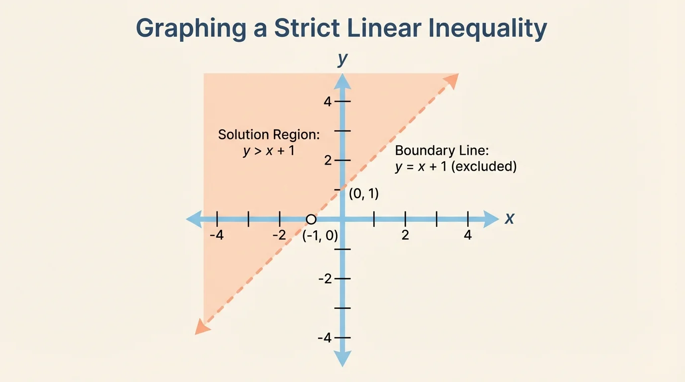
Each ordered pair \((x,y)\) either makes the inequality true or false. The set of all points that make it true is called the solution set. On a graph, that solution set forms one side of a boundary line, as [Figure 1] shows. Because a line divides the coordinate plane into two half-planes, the shaded region is called a half-plane.
For example, in \(y > 2x + 1\), every solution must have a \(y\)-value larger than the line's \(y\)-value at the same \(x\). So all points above the line belong in the graph. Points on the line itself do not belong, because \(y\) is not equal to \(2x + 1\); it must be strictly greater.
Boundary line: the line found by replacing the inequality symbol with an equals sign. For \(y > 2x + 1\), the boundary line is \(y = 2x + 1\).
Strict inequality: an inequality using \(<\) or \(>\). The boundary is not included, so use a dashed line.
Inclusive inequality: an inequality using \(\leq\) or \(\geq\). The boundary is included, so use a solid line.
This distinction between strict and inclusive inequalities matters a lot. The graph is not only about where to shade; it also tells whether points on the line count as solutions.
The process is systematic. Whether the inequality is simple or more complex, the strategy stays almost the same.
Step 1: Find the boundary line by changing the inequality symbol to an equals sign. If needed, rewrite the equation in slope-intercept form \(y = mx + b\) so the line is easier to graph.
Step 2: Decide whether the boundary is dashed or solid. Use a dashed line for \(<\) or \(>\), and a solid line for \(\leq\) or \(\geq\).
Step 3: Determine which side of the line to shade. One common method is to test a point that is not on the line, often \((0,0)\) if it is not on the boundary.
Step 4: Shade the half-plane containing all solutions.
If the inequality is written as \(y > mx + b\), shade above the line. If it is \(y < mx + b\), shade below the line. That shortcut is useful, but the test-point method always works, even when the inequality is in a different form.
Why a test point works
A boundary line divides the plane into two regions. Every point in one region makes the inequality true, and every point in the other region makes it false. Testing a single point tells you which side is the solution side.
If \((0,0)\) is on the boundary line, choose another easy point such as \((1,0)\) or \((0,1)\). The goal is only to identify the correct side, not to find every individual solution one by one.
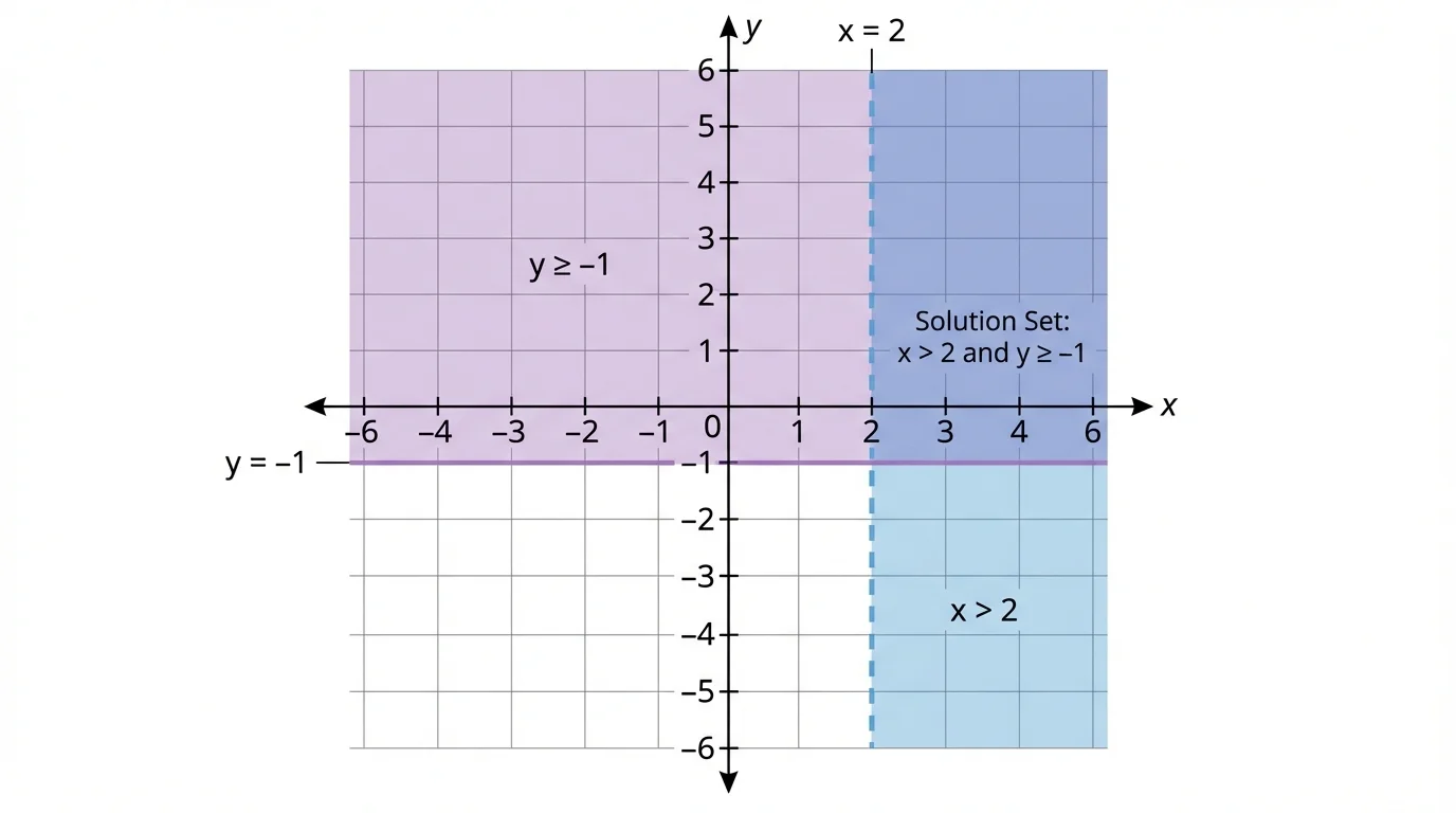
Not every inequality needs to be solved for \(y\) first. Some have especially simple boundary lines, as [Figure 2] illustrates with vertical and horizontal cases.
If the inequality is \(x > 2\), the boundary line is the vertical line \(x = 2\). Since the inequality is strict, the line is dashed, and the region to the right is shaded. If the inequality is \(x \leq 2\), the boundary is solid and the region to the left is shaded.
If the inequality is \(y \geq -1\), the boundary line is the horizontal line \(y = -1\). Because the inequality is inclusive, the line is solid, and the region above it is shaded. Horizontal and vertical inequalities are often the fastest to graph.
Sometimes the inequality is in standard form, such as \(2x + 3y < 12\). You can graph the boundary line \(2x + 3y = 12\) using intercepts or rewrite it as \(y < -\dfrac{2}{3}x + 4\). Either method is correct.
Be careful when solving for \(y\): if you multiply or divide by a negative number, the inequality sign must reverse. For example, from \(-2y > 6x - 8\), dividing by \(-2\) gives \(y < -3x + 4\), not \(y > -3x + 4\).
Now let's work through several examples carefully.
Example 1: Graph \(y > -x + 3\).
Step 1: Identify the boundary line.
Replace \(>\) with \(=\): the boundary line is \(y = -x + 3\).
Step 2: Draw the boundary correctly.
Because the inequality is strict, use a dashed line.
Step 3: Decide which side to shade.
The inequality is \(y > -x + 3\), so shade above the line. To confirm, test \((0,0)\): \(0 > 3\) is false, so the side containing \((0,0)\) is not shaded.
The graph is a dashed line \(y = -x + 3\) with the region above it shaded.
Notice that points on the line, such as \((1,2)\), are not included because they make \(y = -x + 3\), not \(y > -x + 3\).
Example 2: Graph \(2x + y \leq 4\).
Step 1: Rewrite in slope-intercept form.
Subtract \(2x\) from both sides: \(y \leq -2x + 4\).
Step 2: Graph the boundary line.
The boundary is \(y = -2x + 4\). Because the inequality is inclusive, use a solid line.
Step 3: Test a point.
Use \((0,0)\): \(2(0) + 0 \leq 4\) becomes \(0 \leq 4\), which is true.
Step 4: Shade the correct side.
Shade the side containing \((0,0)\). Equivalently, since \(y \leq -2x + 4\), shade below the line.
The graph is the solid line \(y = -2x + 4\) with the region below it shaded.
This is a good example of how a solid line communicates inclusion: any point on \(2x + y = 4\) is part of the solution set.
Example 3: Graph \(x < -3\).
Step 1: Identify the boundary line.
The boundary is the vertical line \(x = -3\).
Step 2: Choose dashed or solid.
Because \(<\) is strict, the boundary is dashed.
Step 3: Shade the correct side.
\(x < -3\) means all points with \(x\)-coordinate less than \(-3\), so shade to the left of the line.
The solution is the half-plane to the left of the dashed line \(x = -3\).
Vertical inequalities are especially useful later in systems, because they can create clear left or right boundaries for a feasible region.
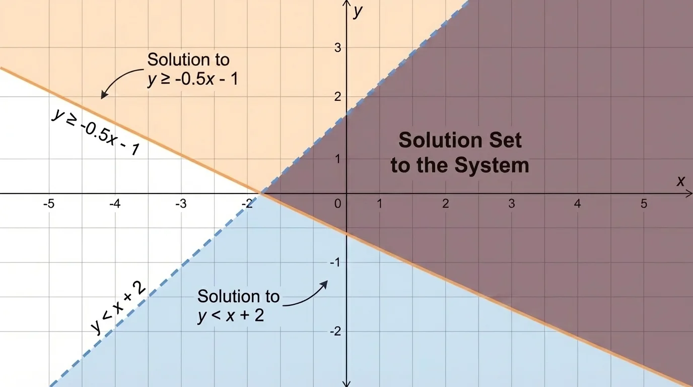
A system of linear inequalities contains two or more inequalities that must all be true at the same time. The solution is the set of points that satisfy every inequality in the system. On a graph, this is the intersection of the corresponding half-planes, as [Figure 3] shows.
To graph a system, graph each inequality separately using the same rules as before. Then look for the region where all the shadings overlap. That overlapping region is the solution set to the entire system.
If no region overlaps, the system has no solution. If the overlap extends forever, the solution set is unbounded. If the overlap forms a closed polygon-like region, that region is often called a feasible region, especially in applications.
Each point in the overlap makes every inequality true. A point outside the overlap may satisfy one inequality but fail another, so it is not a solution to the system.
Systems take the same ideas from single inequalities and combine them.
Example 4: Graph the system \(y \geq x - 1\) and \(y < -x + 3\).
Step 1: Graph the first inequality.
The boundary is \(y = x - 1\). Because the symbol is \(\geq\), draw a solid line and shade above it.
Step 2: Graph the second inequality.
The boundary is \(y = -x + 3\). Because the symbol is \(<\), draw a dashed line and shade below it.
Step 3: Find the overlap.
The solution consists of points that are above or on \(y = x - 1\) and below \(y = -x + 3\).
The solution is the region between the two lines where both conditions hold.
Notice that one boundary is included and one is excluded. That means points on the solid line may count, while points on the dashed line do not.
Example 5: Graph the system \(x \geq 1\), \(y \geq 0\), and \(x + y < 5\).
Step 1: Graph \(x \geq 1\).
Draw the solid vertical line \(x = 1\) and shade to the right.
Step 2: Graph \(y \geq 0\).
Draw the solid horizontal line \(y = 0\) and shade above it.
Step 3: Graph \(x + y < 5\).
Rewrite as \(y < -x + 5\). Draw a dashed line and shade below it.
Step 4: Identify the intersection.
The solution is the region right of \(x = 1\), above \(y = 0\), and below \(y = -x + 5\).
This overlap forms a bounded region. Because one boundary is dashed, the edge on \(x + y = 5\) is not included.
This kind of region appears often in optimization problems, where different constraints limit what combinations are possible.
Example 6: Determine whether \((2,1)\) is a solution to the system \(y > 2x - 4\) and \(y \leq 3\).
Step 1: Test the first inequality.
Substitute \(x = 2\) and \(y = 1\): \(1 > 2(2) - 4\), so \(1 > 0\), which is true.
Step 2: Test the second inequality.
Substitute \(y = 1\): \(1 \leq 3\), which is true.
Step 3: State the result.
Because the point satisfies both inequalities, \((2,1)\) is in the solution set.
Checking points directly is a powerful way to verify whether a graphed region makes sense.
Later, as seen again in [Figure 3], the most important visual feature of a system is not each separate shading by itself, but the overlap that survives all conditions at once.
One very common mistake is drawing the wrong type of boundary line. Remember: \(<\) and \(>\) mean dashed; \(\leq\) and \(\geq\) mean solid.
Another common mistake is shading the wrong side. If you are unsure, use a test point. This is safer than relying only on memory.
A third mistake happens when solving for \(y\). If you divide by a negative number, reverse the inequality symbol. Missing that step changes the entire graph.
Students also sometimes think the solution to a system is the union of all shaded parts. It is not. The solution is only the overlap, the region where every inequality is true simultaneously.
| Inequality type | Boundary | Shading idea |
|---|---|---|
| \(y > mx + b\) | dashed | above the line |
| \(y \geq mx + b\) | solid | above the line |
| \(y < mx + b\) | dashed | below the line |
| \(y \leq mx + b\) | solid | below the line |
| \(x > a\) or \(x \geq a\) | vertical line | right of the line |
| \(x < a\) or \(x \leq a\) | vertical line | left of the line |
Table 1. A quick comparison of boundary-line style and shading direction for common forms of linear inequalities.
Linear inequalities are not just graphing exercises. They model restrictions. A company may need to keep cost below a certain amount, produce at least a minimum number of items, or stay within available labor hours. Each restriction can be written as an inequality, and the graph shows all possible choices.
Suppose a school event can sell adult tickets \(x\) and student tickets \(y\). If there must be at least \(100\) tickets sold, then \(x + y \geq 100\). If the venue holds at most \(180\) people, then \(x + y \leq 180\). If at least \(40\) adult tickets are needed, then \(x \geq 40\). The solution region consists of all ticket combinations that satisfy every condition.
In manufacturing, one product may require \(2\) hours of machine time and another may require \(3\) hours. If only \(60\) machine hours are available, then \(2x + 3y \leq 60\). If both products must be nonnegative in quantity, then \(x \geq 0\) and \(y \geq 0\). The resulting feasible region helps managers compare realistic production plans.
Airlines, delivery companies, and factories often use systems of inequalities behind the scenes. Before finding the "best" plan, they first identify which plans are even possible.
The same visual idea appears in economics, engineering, and computer science: acceptable choices form a region, and the boundary lines mark limits that may be included or excluded, depending on the inequality.