Some of the most important patterns in science and technology are not straight lines. Bacteria can double in number, earthquake intensity is measured on a logarithmic scale, and sound, light, tides, and electricity rise and fall in repeating waves. The graphs of these functions are powerful because they reveal how a quantity behaves over time: whether it explodes upward, levels off, drops rapidly, or repeats in cycles.
When you graph a function, you are doing more than plotting points. You are reading a story about change. For exponential and logarithmic functions, the story often involves very fast growth or very slow response. For trigonometric functions, the story involves periodic behavior. Understanding intercepts, end behavior, period, midline, and amplitude helps you predict what happens before and after the visible part of the graph.
These ideas also connect algebra to graphing. If you can read a formula like \(y = 3(2)^x - 1\), \(y = \log_2(x-4) + 3\), or \(y = 2\sin(3x) + 1\), you can predict the graph's shape and key features without needing a calculator for every point.
From earlier graphing work, remember that an intercept is where a graph crosses an axis. A y-intercept occurs when \(x = 0\), and an x-intercept occurs when \(y = 0\). Also remember that a transformation can shift, stretch, compress, or reflect a basic parent function.
An exponential graph, a logarithmic graph, and a trigonometric graph may look very different, but all of them can be understood by starting from a parent function and then analyzing how parameters change that parent shape.
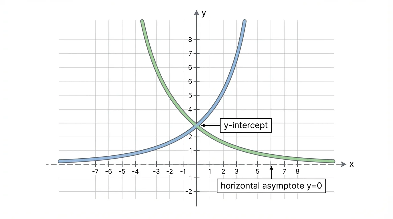
[Figure 1] A exponential function has a variable in the exponent, usually written in a form such as \[y = ab^x + k\] where \(a \neq 0\), \(b > 0\), and \(b \neq 1\). The number \(b\) is called the base. If \(b > 1\), the function shows exponential growth. If \(0 < b < 1\), it shows exponential decay. One of the most important visual ideas is that exponential graphs approach a horizontal line but do not usually cross it.
For the parent function \(y = b^x\), the graph passes through \((0,1)\) because \(b^0 = 1\). That means the y-intercept is \((0,1)\). There is no x-intercept because \(b^x\) is always positive. The horizontal asymptote is \(y = 0\). The domain is all real numbers, and the range is \(y > 0\).
The end behavior depends on the base. If \(y = 2^x\), then as \(x \to \infty\), \(y \to \infty\), and as \(x \to -\infty\), \(y \to 0\). If \(y = \left(\dfrac{1}{2}\right)^x\), then as \(x \to \infty\), \(y \to 0\), and as \(x \to -\infty\), \(y \to \infty\).
Transformations change these features. In \(y = ab^x + k\), the value of \(k\) shifts the graph up or down and changes the horizontal asymptote from \(y = 0\) to \(y = k\). The factor \(a\) stretches the graph vertically and reflects it across the x-axis if \(a < 0\).
A horizontal asymptote is a horizontal line that a graph approaches as \(x\) becomes very large positive or very large negative.
Growth means the function's values increase multiplicatively over equal input intervals, while decay means the values decrease multiplicatively over equal input intervals.
For example, consider \(y = 3(2)^x - 6\). The horizontal asymptote is \(y = -6\). The y-intercept is found by substituting \(x = 0\): \(y = 3(2)^0 - 6 = 3 - 6 = -3\), so the y-intercept is \((0,-3)\). To find the x-intercept, set \(y = 0\): \(0 = 3(2)^x - 6\), so \(3(2)^x = 6\), then \(2^x = 2\), so \(x = 1\). The x-intercept is \((1,0)\).
Notice how much information came from the equation alone: intercepts, asymptote, and end behavior. This is why symbolic and graphical representations are so closely connected.
A good way to sketch exponential functions by hand is to begin with the parent graph \(y = b^x\), then apply transformations. For \(y = -2\left(\dfrac{1}{3}\right)^x + 4\), the parent function is exponential decay because the base \(\dfrac{1}{3}\) lies between \(0\) and \(1\). Then the factor \(-2\) reflects the graph across the x-axis and stretches it vertically. Finally, the \(+4\) shifts everything up by \(4\), making \(y = 4\) the horizontal asymptote.
To locate the y-intercept, use \(x = 0\): \(y = -2\left(\dfrac{1}{3}\right)^0 + 4 = -2 + 4 = 2\). So the graph crosses the y-axis at \((0,2)\). To understand its ends, observe that as \(x \to \infty\), \(\left(\dfrac{1}{3}\right)^x \to 0\), so \(y \to 4\). As \(x \to -\infty\), \(\left(\dfrac{1}{3}\right)^x\) becomes very large, and multiplying by \(-2\) makes \(y\) fall without bound.
Later, when comparing models, the exponential graphs help you recognize a key pattern: exponential functions change quickly at first, then either surge upward or flatten toward an asymptote.
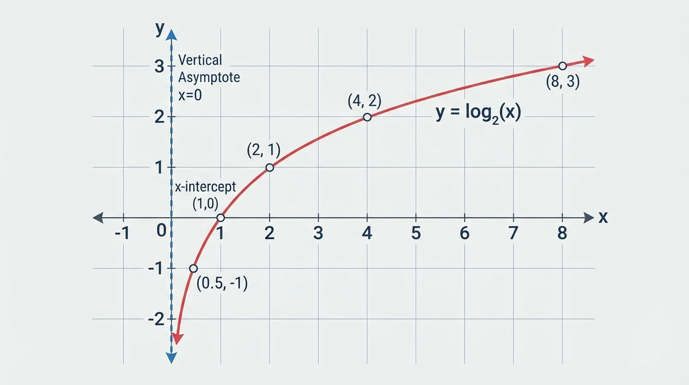
[Figure 2] A logarithmic function is the inverse of an exponential function. A common form is \[y = \log_b(x)\] where \(b > 0\) and \(b \neq 1\). An exponential function gives the output for a given input, while a logarithmic function gives the exponent needed to produce a given output. Logarithmic graphs behave very differently: they are restricted to one side of a vertical asymptote.
For the parent function \(y = \log_b(x)\), the domain is \(x > 0\), because you cannot take the logarithm of a nonpositive number in the real-number system. The range is all real numbers. The graph has a vertical asymptote at \(x = 0\). The x-intercept occurs at \((1,0)\), because \(\log_b(1) = 0\). There is no y-intercept, since the function is not defined at \(x = 0\).
The end behavior also matters. If \(y = \log_b(x)\) with \(b > 1\), then as \(x \to \infty\), \(y \to \infty\), and as \(x \to 0^+\), \(y \to -\infty\). If \(0 < b < 1\), the graph decreases instead of increases.
Transformations work much like they do for other functions. In \(y = \log_2(x-3) + 1\), the graph of \(y = \log_2(x)\) shifts right by \(3\) and up by \(1\). That moves the vertical asymptote from \(x = 0\) to \(x = 3\). The x-values in the domain must satisfy \(x - 3 > 0\), so the domain is \(x > 3\).
Why logarithms grow slowly
Exponential functions can explode upward because each increase in \(x\) multiplies the output. Logarithmic functions reverse that process. To increase the logarithm by just \(1\), the input must be multiplied by the base. That is why a logarithmic graph rises, but more and more slowly.
For \(y = \log_2(x-3) + 1\), the x-intercept is found by setting \(y = 0\): \(0 = \log_2(x-3) + 1\), so \(-1 = \log_2(x-3)\). Rewriting in exponential form gives \(x - 3 = 2^{-1} = \dfrac{1}{2}\), so \(x = \dfrac{7}{2}\). The x-intercept is \(\left(\dfrac{7}{2},0\right)\). There is still no y-intercept because \(x = 0\) is outside the domain.
[Figure 3] Because logarithmic and exponential functions are inverses, their graphs are reflections across the line \(y = x\). This relationship is one of the clearest ways to connect symbolic equations to graph shapes.
If \(y = 2^x\), then its inverse is \(y = \log_2(x)\). The point \((0,1)\) on the exponential graph becomes \((1,0)\) on the logarithmic graph. The horizontal asymptote \(y = 0\) for the exponential becomes the vertical asymptote \(x = 0\) for the logarithm.
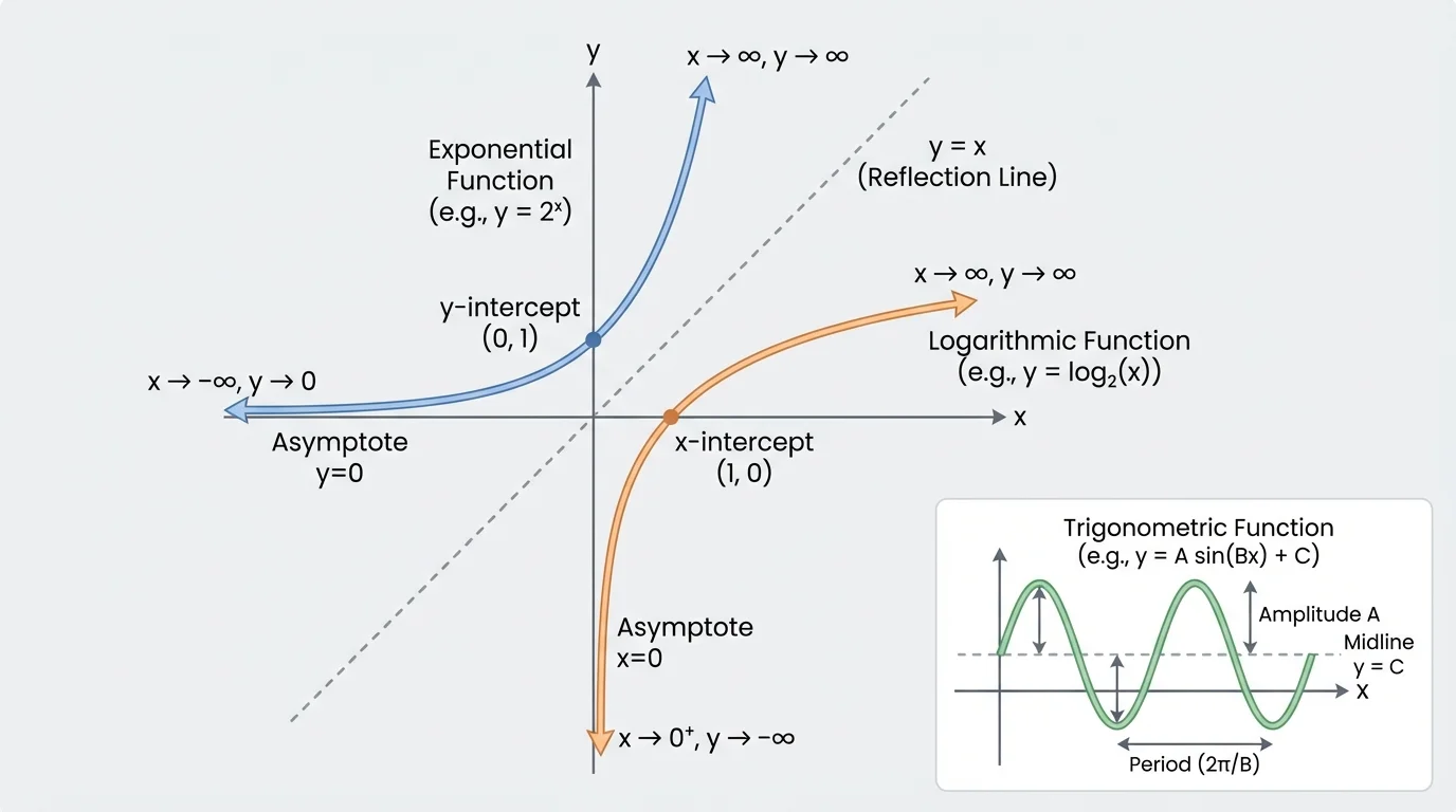
This inverse relationship helps you solve equations and understand graph behavior. For instance, if \(2^x = 7\), then \(x = \log_2(7)\). Graphically, that means the y-value \(7\) on the exponential corresponds to the x-value \(7\) on the logarithmic graph after reflection across \(y = x\).
When students confuse these two function families, the reflected shapes often make the difference clear: exponential graphs are defined for every real \(x\), while logarithmic graphs are only defined for positive inputs after accounting for transformations.
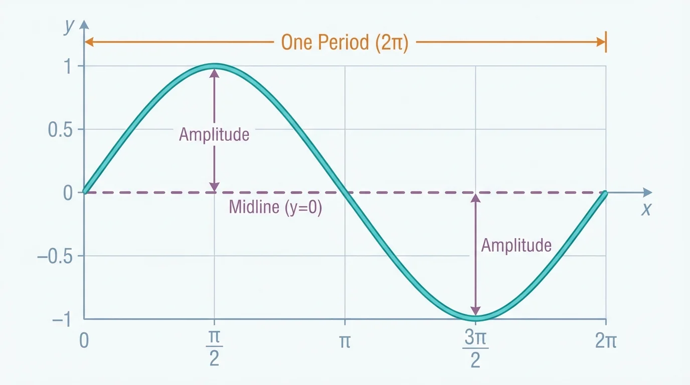
[Figure 4] A trigonometric function models repeating patterns. The most common graphs at this level are sine and cosine. A general sinusoidal form is \[y = a\sin(bx) + d \quad \textrm{or} \quad y = a\cos(bx) + d\] where \(a\) controls the amplitude, \(b\) controls the period, and \(d\) sets the midline. These three features are the first things to identify when reading a trigonometric graph.
The amplitude is the distance from the midline to a peak or to a trough. For \(y = a\sin(bx) + d\), the amplitude is \(|a|\). The midline is the horizontal line \(y = d\). The period tells how long one complete cycle lasts. For sine and cosine, the period is \[\frac{2\pi}{|b|}\]
The parent functions are \(y = \sin(x)\) and \(y = \cos(x)\). Both have amplitude \(1\), period \(2\pi\), and midline \(y = 0\). The sine graph starts at \((0,0)\), rises to \((\dfrac{\pi}{2},1)\), returns to \((\pi,0)\), falls to \((\dfrac{3\pi}{2},-1)\), and returns to \((2\pi,0)\). The cosine graph starts at a maximum point \((0,1)\).
If \(a < 0\), the graph reflects across the midline. If \(|a| > 1\), the wave gets taller. If \(|b| > 1\), the graph is compressed horizontally, so the period becomes shorter. If \(0 < |b| < 1\), the graph stretches horizontally, so the period becomes longer.
Amplitude is half the distance between the maximum and minimum values of a sinusoidal graph.
Period is the length of one complete cycle.
Midline is the horizontal line halfway between the maximum and minimum values.
For example, in \(y = 3\sin(2x) - 1\), the amplitude is \(3\), the period is \(\dfrac{2\pi}{2} = \pi\), and the midline is \(y = -1\). The maximum value is \(-1 + 3 = 2\), and the minimum value is \(-1 - 3 = -4\).
To sketch a sinusoidal graph, identify the midline, amplitude, and period first. Then divide one period into four equal parts. This works because sine and cosine can be drawn using five key points over one cycle: the starting point, the first quarter-point, the halfway point, the third quarter-point, and the endpoint.
For \(y = 2\cos\left(\dfrac{1}{2}x\right) + 3\), the amplitude is \(2\), the midline is \(y = 3\), and the period is \(\dfrac{2\pi}{1/2} = 4\pi\). One cycle can be marked from \(x = 0\) to \(x = 4\pi\). Since cosine begins at a maximum, the five key points are \((0,5)\), \((\pi,3)\), \((2\pi,1)\), \((3\pi,3)\), and \((4\pi,5)\).
The labeled wave helps show why amplitude and period are different ideas: amplitude measures vertical size, while period measures horizontal length.
| Function form | Key feature | How to find it |
|---|---|---|
| \(y = ab^x + k\) | Horizontal asymptote | \(y = k\) |
| \(y = ab^x + k\) | Y-intercept | Substitute \(x = 0\) |
| \(y = \log_b(x-h) + k\) | Vertical asymptote | \(x = h\) |
| \(y = \log_b(x-h) + k\) | Domain | \(x > h\) |
| \(y = a\sin(bx) + d\) or \(y = a\cos(bx) + d\) | Amplitude | \(|a|\) |
| \(y = a\sin(bx) + d\) or \(y = a\cos(bx) + d\) | Period | \(\dfrac{2\pi}{|b|}\) |
| \(y = a\sin(bx) + d\) or \(y = a\cos(bx) + d\) | Midline | \(y = d\) |
Table 1. Key graph features for exponential, logarithmic, and sinusoidal functions.
Worked examples make the graphing process more visible. Notice how each step connects the equation to a graph feature.
Worked example 1: Graph an exponential function
Find the asymptote, intercepts, and end behavior of \(y = 2\left(\dfrac{1}{2}\right)^x + 1\).
Step 1: Identify the transformation.
The parent function is \(y = \left(\dfrac{1}{2}\right)^x\), which is exponential decay. The \(+1\) shifts the graph up by \(1\).
Step 2: Find the horizontal asymptote.
Since the graph is shifted up by \(1\), the asymptote is \(y = 1\).
Step 3: Find the y-intercept.
Substitute \(x = 0\): \(y = 2\left(\dfrac{1}{2}\right)^0 + 1 = 2(1) + 1 = 3\). So the y-intercept is \((0,3)\).
Step 4: Check for an x-intercept.
Set \(y = 0\): \(0 = 2\left(\dfrac{1}{2}\right)^x + 1\). Then \(2\left(\dfrac{1}{2}\right)^x = -1\), which is impossible because \(2\left(\dfrac{1}{2}\right)^x\) is always positive. So there is no x-intercept.
Step 5: Describe end behavior.
As \(x \to \infty\), \(\left(\dfrac{1}{2}\right)^x \to 0\), so \(y \to 1\). As \(x \to -\infty\), the output grows without bound, so \(y \to \infty\).
The graph is a decay curve above the line \(y = 1\), crossing the y-axis at \((0,3)\).
This example shows that exponential graphs do not always cross the x-axis. A vertical shift can move the entire graph above or below the axis.
Worked example 2: Graph a logarithmic function
Find the vertical asymptote, domain, and x-intercept of \(y = \log_3(x+2) - 2\).
Step 1: Find the asymptote from the input.
The logarithm's input is \(x+2\). Set it equal to \(0\): \(x + 2 = 0\), so the vertical asymptote is \(x = -2\).
Step 2: Find the domain.
The input of a logarithm must be positive: \(x + 2 > 0\), so \(x > -2\).
Step 3: Find the x-intercept.
Set \(y = 0\): \(0 = \log_3(x+2) - 2\). Then \(2 = \log_3(x+2)\). Rewrite in exponential form: \(x + 2 = 3^2 = 9\). Therefore \(x = 7\).
Step 4: State the intercept.
The x-intercept is \((7,0)\).
The graph increases slowly to the right and drops toward negative infinity as it approaches \(x = -2\) from the right.
The asymptote and domain come directly from the expression inside the logarithm. This is one of the fastest ways to sketch a log graph.
Worked example 3: Analyze a trigonometric function
For \(y = -4\cos(3x) + 2\), find the amplitude, period, midline, maximum value, and minimum value.
Step 1: Identify the parameters.
Here \(a = -4\), \(b = 3\), and \(d = 2\).
Step 2: Find the amplitude.
Amplitude is \(|a| = |-4| = 4\).
Step 3: Find the period.
Period is \(\dfrac{2\pi}{|b|} = \dfrac{2\pi}{3}\).
Step 4: Find the midline.
The midline is \(y = d = 2\).
Step 5: Find maximum and minimum values.
Maximum value is \(2 + 4 = 6\). Minimum value is \(2 - 4 = -2\).
The negative sign reflects the cosine graph across its midline, but it does not change the amplitude.
A common mistake is to call \(-4\) the amplitude. Amplitude is always nonnegative, so we use \(|a|\).
The Richter scale for earthquakes and the decibel scale for sound use logarithms, while alternating current in electrical systems is modeled by sine and cosine waves. Different graph families describe different kinds of real phenomena, but they often work together in science and engineering.
Another useful comparison is that exponential and logarithmic functions are often used when change is multiplicative, while trigonometric functions are used when change is cyclical.
Exponential functions appear in population growth, radioactive decay, compound interest, and the spread of information online. If an amount doubles every hour, the graph is exponential growth. If a medicine is removed from the bloodstream by a constant percentage each hour, the graph is exponential decay.
Logarithmic functions appear whenever humans need to compress huge ranges into manageable scales. For example, pH values, earthquake magnitudes, and sound intensity are all based on logarithms. A small change on the graph may represent a very large change in the actual quantity.
Trigonometric functions model periodic behavior such as tides, daylight hours, Ferris wheel motion, sound waves, and electrical signals. In these situations, the amplitude tells how far the quantity moves from its average value, the midline represents that average value, and the period tells how long one cycle takes.
Suppose a city's average temperature through a season is modeled by \(T(t) = 8\sin\left(\dfrac{\pi}{6}t\right) + 15\), where \(t\) is measured in months. The amplitude \(8\) means temperatures vary \(8\) degrees above and below the average. The midline \(15\) means the average temperature is \(15\). The period is \(\dfrac{2\pi}{\pi/6} = 12\), so the cycle repeats every \(12\) months.
Seeing these graphs as models makes the features meaningful. An asymptote might represent a limiting value. An intercept may represent an initial amount or a threshold. A midline may represent equilibrium, and a period may represent a repeating schedule.
"Mathematics reveals its power when a graph turns an equation into a visible pattern."
Whether you are studying finance, chemistry, music, or engineering, these graph features help you interpret how quantities change and what the symbols in an equation really mean.