A graph is more than a picture of lines and curves. It can show when a population grows fastest, when a business earns the most money, when a car is stopped, or when a medicine reaches its strongest effect. When a function models a relationship between two quantities, every important point and pattern on its graph tells part of a story. Learning to read that story is one of the most useful skills in algebra, because it connects mathematics to the real world.
Suppose a graph shows the height of a basketball after it is thrown. A high point on the graph is not just a "maximum" in abstract mathematical language; it represents the highest point the ball reaches. An interval where the graph falls means the ball is coming down. A point where the graph meets the horizontal axis may represent the moment the ball hits the ground. Interpreting functions means translating mathematical features into meaning about the quantities involved.
In many applications, one quantity depends on another. If time is the input, then output might be height, distance, temperature, cost, pressure, or population. A function gives exactly one output for each input in its domain. The graph, table, and verbal description are different ways of representing the same relationship.
Key features of a function are the important parts of its graph or table that help explain the relationship between the quantities. These often include the domain, range, intercepts, intervals where the function is increasing or decreasing, relative maxima and minima, and end behavior.
In context, these features should always be interpreted with units and meaning. For example, saying "the function has a maximum at \((4, 70)\)" is incomplete. A better interpretation is: "After \(4\) hours, the temperature reaches a maximum of \(70^\circ\textrm{F}\)." The mathematics identifies the feature, but the context explains why it matters.
[Figure 1] Several graph features appear again and again in applications. The horizontal axis usually represents the independent variable, or input, and the vertical axis represents the dependent variable, or output.
The domain is the set of allowable input values. The range is the set of resulting output values. In pure algebra, the domain and range may include many values, but in applications they are often restricted. If a function models the number of tickets sold, negative numbers of tickets sold do not make sense. If a function models the height of a person over time, the time variable might begin at birth, not at a negative number of years.
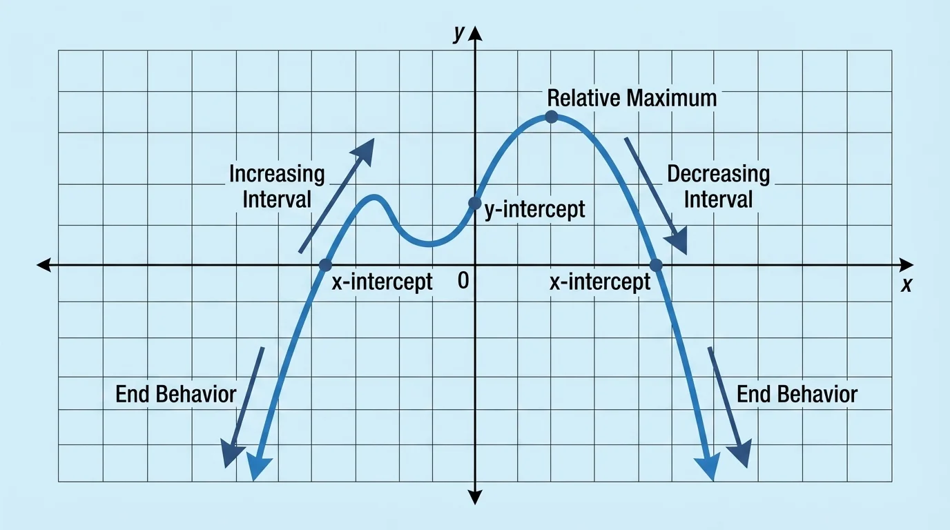
An intercept is where a graph meets an axis. A y-intercept occurs when \(x = 0\), so it tells the starting value of the output. A x-intercept occurs when \(y = 0\), so it tells when the output becomes zero. In a cost graph, the y-intercept may represent a starting fee. In a height graph, an x-intercept may represent when an object reaches the ground.
An interval where the function is increasing means the output rises as the input increases. An interval where it is decreasing means the output falls as the input increases. Be careful: increasing does not describe the input changing; the input usually moves left to right. It describes what happens to the output as the input increases.
A relative maximum is a point where the function has a higher value than nearby points. A relative minimum is a point where the function has a lower value than nearby points. In context, these often represent "highest so far" or "lowest so far" situations, such as maximum profit, peak heart rate, or minimum fuel level during a trip.
End behavior describes what happens to the graph as the input values become very large positive or very large negative numbers, when that makes sense in the context. In an application, end behavior may have limited meaning if the model only applies over a certain interval. For example, a model for a plant's height may be meaningful for \(0 \le x \le 100\) days, but not for all real numbers.
When you look back at [Figure 1], notice that each feature answers a different kind of question: where the relationship starts, where it reaches zero, where it rises or falls, and where it reaches high or low points. That is why graph interpretation is so powerful: one picture can communicate many ideas at once.
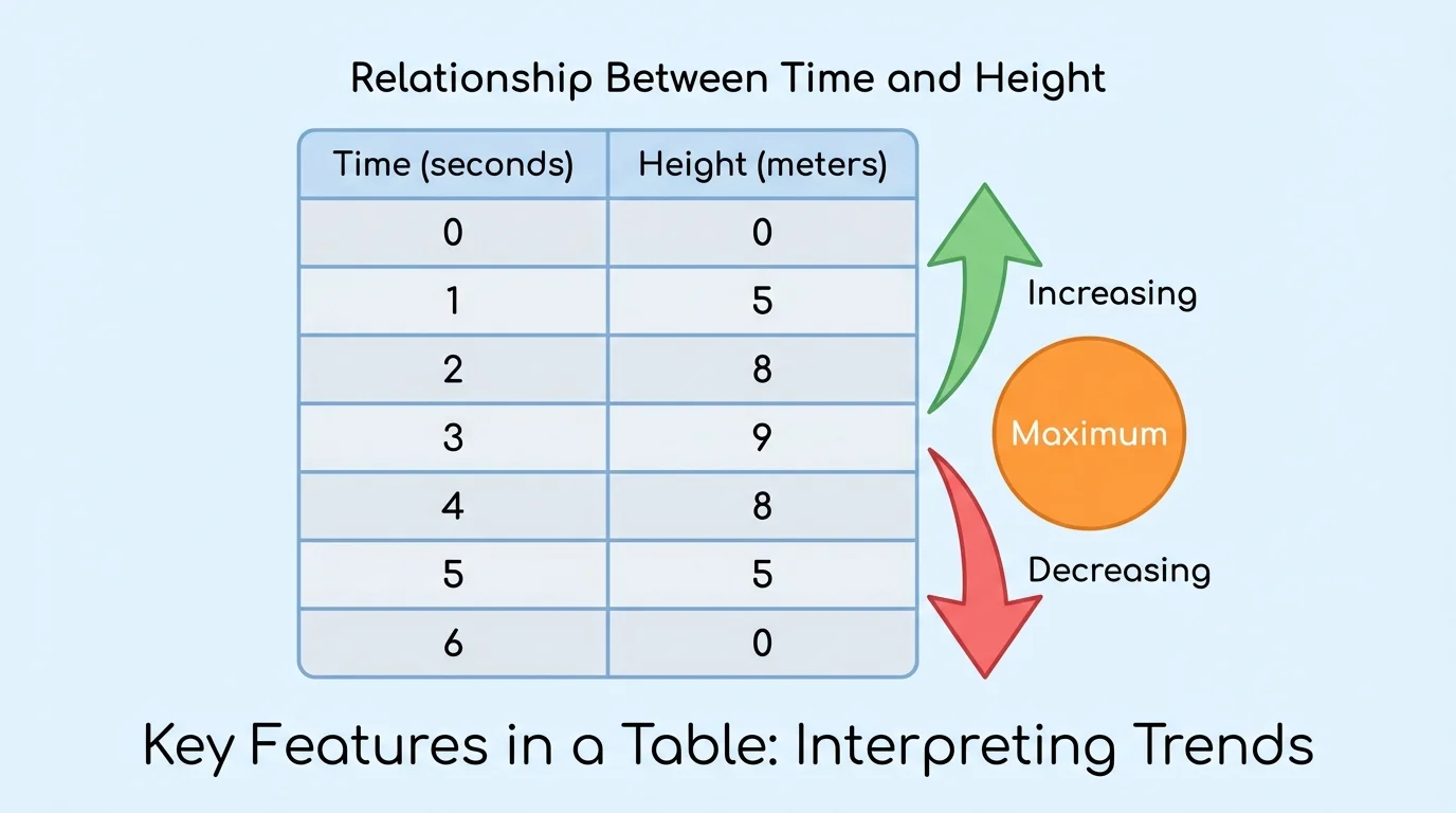
[Figure 2] A graph is not the only way to interpret a function. A table can reveal the same key features, and repeated changes in a table can show trends such as increasing, decreasing, or reaching a peak.
When reading a table, begin by identifying what each column represents. Then compare outputs as the inputs increase. If the outputs get larger, the function is increasing over that interval. If the outputs get smaller, the function is decreasing. If the outputs change direction, a maximum or minimum may be near that input value.
Tables can also show intercepts. If the table includes \(x = 0\), then the corresponding output is the \(y\)-intercept. If some output value is \(0\), then the corresponding input gives an \(x\)-intercept. Sometimes the exact intercept is not listed, but the table can still suggest where it occurs. For example, if the output changes from positive to negative between two rows, the graph likely crosses the horizontal axis between those inputs.
Tables are especially useful when data come from measurements. Scientists, economists, and engineers often start with tables before creating graphs. But tables have limits: they show only selected values, not the full shape between them. That is why it is important to infer patterns carefully rather than assume too much.
To interpret a table well, recall that a function pairs each input with exactly one output. If a table gave the same input with two different outputs, it would not represent a function.
A table can also hint at the type of function. Constant first differences may suggest a linear relationship. Outputs that rise to a highest point and then fall may suggest a quadratic pattern. Rapid growth by repeated multiplication may suggest exponential behavior. These patterns help when you later sketch a graph from data.
Context changes everything. The same graph shape can mean very different things depending on what the variables represent. A rising line could show increasing earnings, growing rainfall totals, or a car moving farther from home at a constant speed. The shape alone is not enough; the axis labels and units matter.
For example, if a graph shows distance from home versus time, a horizontal segment means the distance is not changing. That does not mean time has stopped. It means the person is staying in one place. If a graph shows temperature versus time, a horizontal segment means the temperature remains constant. If a graph shows speed versus time, a horizontal segment means the speed stays the same.
Negative outputs may or may not make sense in context. A graph of elevation relative to sea level can have negative values. A graph of the number of students in a classroom cannot. Likewise, a steep graph does not always mean "high"; it often means "changing quickly." Steepness relates to rate of change, not just to the output value itself.
Interpreting in context means answering with meaning, not just coordinates. When you identify a point such as \((5, 200)\), always ask: what does the input \(5\) represent, and what does the output \(200\) represent? A complete interpretation might be: "After \(5\) minutes, the machine has produced \(200\) parts."
This habit is essential in advanced mathematics and in professional practice. A scientist, coach, engineer, or business analyst does not just say that a graph increases; they explain what is increasing and why that matters.
A table shows the percentage of battery charge remaining on a phone during a school day.
| Time after \(0\) hours | Battery percentage |
|---|---|
| \(0\) | \(100\) |
| \(1\) | \(92\) |
| \(2\) | \(83\) |
| \(3\) | \(71\) |
| \(4\) | \(58\) |
Worked example
Interpret the key features of the table.
Step 1: Identify the variables.
The input is time in hours, and the output is battery percentage.
Step 2: Find the starting value.
At \(x = 0\), the battery percentage is \(100\). So the \(y\)-intercept is \((0, 100)\), meaning the phone starts fully charged.
Step 3: Describe whether the function increases or decreases.
The outputs go from \(100\) to \(92\) to \(83\) to \(71\) to \(58\). Since the outputs decrease as time increases, the function is decreasing over the interval shown.
Step 4: Interpret the rate qualitatively.
The battery does not drop by exactly the same amount each hour, but it steadily loses charge. There is no maximum after the start and no minimum listed yet, though \(58\) is the lowest value shown.
A good contextual interpretation is: "The phone battery starts at \(100\%\) and steadily decreases during the first \(4\) hours of the day."
This example shows that a table can provide a clear story even without a graph. It tells the initial amount, the trend, and the practical meaning of the change.
A school theater group graphs profit as a function of ticket price. The graph rises, reaches a maximum point at \((8, 960)\), and then falls. It crosses the horizontal axis at \((2, 0)\) and \((14, 0)\).
Worked example
Interpret the important features of this graph.
Step 1: Interpret the intercepts.
The points \((2, 0)\) and \((14, 0)\) are \(x\)-intercepts. This means if the ticket price is \(\$2\) or \(\$14\), the profit is \(\$0\).
Step 2: Interpret the maximum point.
The point \((8, 960)\) is the highest point on the graph. So when the ticket price is \(\$8\), the theater group earns a maximum profit of \(\$960\).
Step 3: Describe increasing and decreasing intervals.
As ticket price increases from \(\$2\) to \(\$8\), profit increases. As ticket price increases from \(\$8\) to \(\$14\), profit decreases.
Step 4: Explain the meaning in context.
Very low ticket prices do not bring enough money per ticket, and very high ticket prices may reduce attendance. A middle price gives the greatest profit.
The key interpretation is that the best ticket price, according to this model, is \(\$8\).
This kind of graph appears in business, economics, and event planning. The goal is not only to identify the maximum but to explain what decision it supports.
A verbal description can be turned into a graph when you track how one quantity changes with another. Consider this situation: "A student walks away from home at a steady pace for \(10\) minutes, waits at a friend's house for \(20\) minutes, and then returns home faster than before."
Worked example
[Figure 3] Sketch and interpret the graph of distance from home as a function of time.
Step 1: Identify the variables.
The input is time, and the output is distance from home.
Step 2: Graph the first part of the story.
Walking away from home at a steady pace means distance increases at a constant rate. Sketch an upward-sloping line from the origin over the first \(10\) minutes.
Step 3: Graph the waiting period.
Waiting at the friend's house means distance from home stays constant. Sketch a horizontal segment for the next \(20\) minutes.
Step 4: Graph the return trip.
Returning home faster means distance decreases to \(0\) at a steeper rate than it increased before. Sketch a downward line segment that reaches the horizontal axis.
The graph starts by rising, stays flat, and then falls more steeply back to zero.
The shape matters. An upward line means moving away, a flat segment means staying put, and a downward line means returning. The steeper downward segment shows a faster speed on the way back.
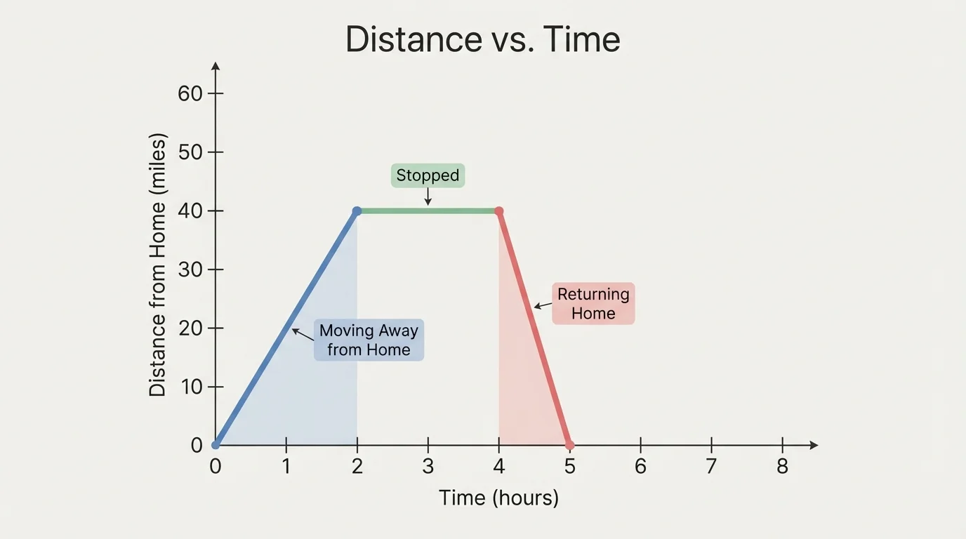
You can see that the graph does not show the student's path on a map. It shows how distance changes over time. That distinction is crucial: function graphs describe relationships between variables, not physical shapes of motion through space.
[Figure 4] Some graph shapes appear so often that they become useful visual clues. Recognizing these does not replace interpretation, but it helps you make sense of a model quickly.
A linear function has a straight-line graph. In context, it often represents a constant rate of change, such as earning the same amount per hour or traveling at a constant speed. A quadratic function often rises to a peak and then falls, or falls to a low point and then rises. Projectile motion and area optimization problems often behave this way.
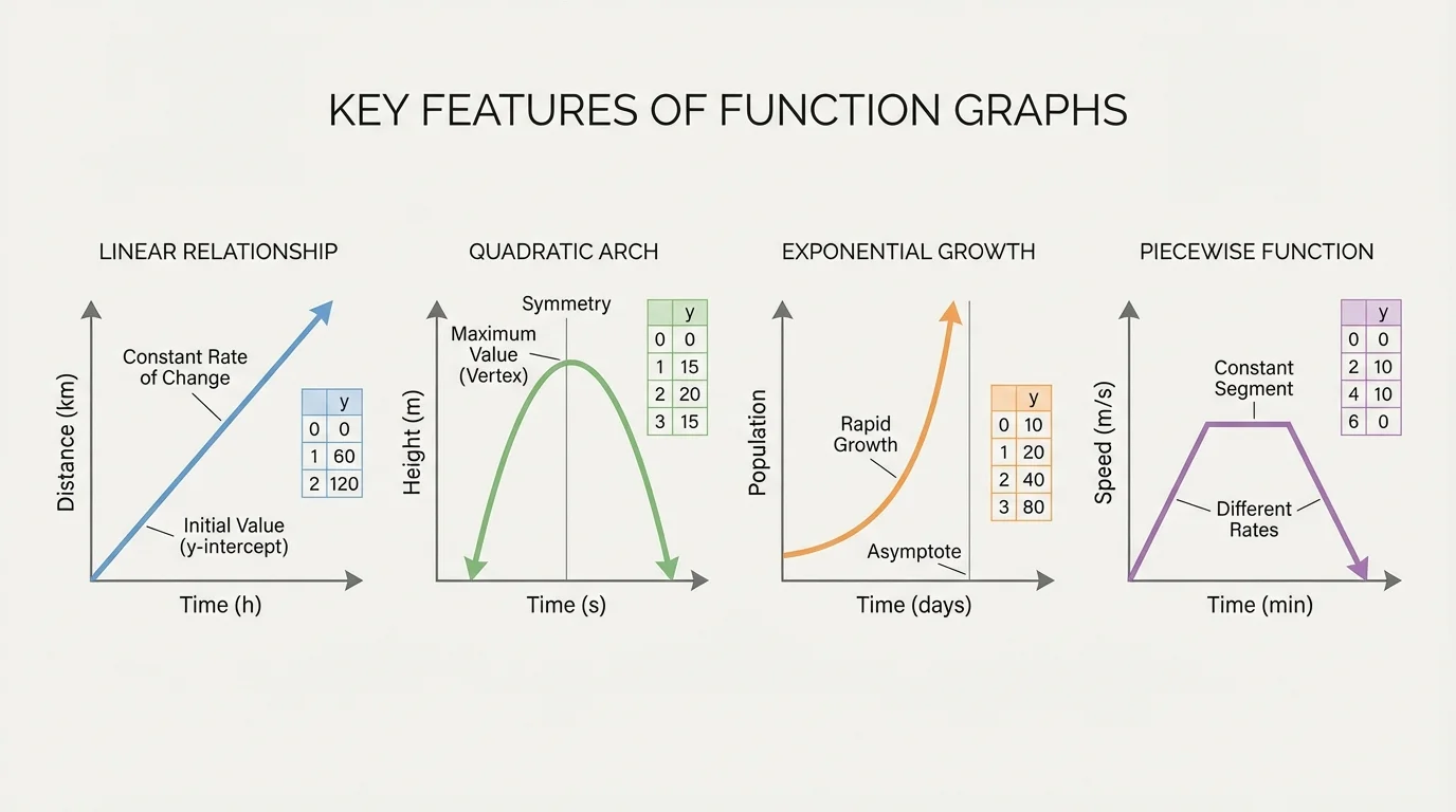
An exponential function changes by repeated multiplication rather than repeated addition. It often models population growth, compound interest, or radioactive decay. A piecewise function uses different rules on different intervals. In real life, this is common when conditions change, such as different taxi pricing rules or a trip with stops.
The shapes are different, but each one suggests a different kind of story: constant change, rise-and-fall behavior, rapid growth, or rule changes across intervals. Interpreting functions well means connecting those shapes to situations.
Modern apps use function graphs constantly. Fitness trackers, battery monitors, stock charts, and weather forecasts all rely on interpreting changing quantities over time.
In science, a graph of temperature versus time can show when a substance heats up, stays at a constant temperature during a phase change, and then heats again. In medicine, a graph of drug concentration in the bloodstream can show when a medication reaches peak effectiveness and when it begins to wear off.
In economics, graphs of cost, revenue, and profit help businesses choose prices and production levels. In sports, a graph of speed versus time can reveal acceleration, rest periods, and fatigue. In environmental studies, graphs of carbon dioxide concentration, rainfall, or sea level help researchers identify long-term trends and turning points.
These applications all use the same mathematical habits: identify what each axis means, find important features, and explain those features in words tied to the situation. The graph is only useful if its features are interpreted correctly.
"The most important thing about a graph is not what it looks like, but what it means."
One common mistake is confusing a graph's shape with a real path. For example, a graph of a person's distance from home over time is not a picture of the road the person walks on. It is a record of how distance changes.
Another mistake is naming a feature without interpreting it. Saying "there is a maximum at \((6, 120)\)" is not enough. You should explain that "after \(6\) minutes, the value reaches \(120\)," and then identify what those quantities represent.
Students also sometimes ignore domain restrictions. A model may have a graph that continues forever, but the real situation may not. If a graph models water in a tank as it drains, negative time or negative water volume may not make sense. The realistic domain matters.
Finally, be careful with tables. A table shows discrete values, not every value in between. You can infer trends, but you should not claim exact features unless the information supports them.
When you face a graph, table, or verbal description, use a simple strategy. First, identify the two quantities and their units. Second, determine which quantity depends on the other. Third, look for starting values, zeroes, rising or falling intervals, highest or lowest points, and any unusual behavior such as flat segments or sudden changes. Fourth, translate each feature into a sentence about the situation.
When sketching from words, think in pieces. Ask: Is the output increasing, decreasing, or staying the same? Is the change steady or curved? Does the graph start at zero, above zero, or below zero? Is there a turning point? These questions turn a verbal story into a visual model.
Interpreting functions is one of the clearest examples of mathematics as a language. Graphs and tables are not just collections of values. They are compact ways to describe how the world changes.