A graph can reveal a surprising amount about a formula before you ever compute many values. A square root graph begins at a single point and grows slowly. A cube root graph stretches across all real numbers but flattens and steepens in a very different way. In a piecewise-defined function, the rule can suddenly switch at a particular input value, which means one graph can look like several graphs joined together. Learning to read these shapes is one of the fastest ways to understand how functions behave.
In algebra, a function is not just an equation to simplify. It is also a relationship you can see. When you graph a function, you can identify where it starts, how quickly it changes, where it is defined, and whether it has jumps, corners, or smooth curves. These visual features matter in science, engineering, economics, and technology because real systems often do not behave in one perfectly smooth way.
Some functions are built from roots. Others are built from different rules on different intervals. This lesson focuses on three important types: square root functions, cube root functions, and functions that use separate formulas depending on the value of x.
Recall that the domain of a function is the set of input values for which the function is defined, and the range is the set of output values. When graphing by hand, always ask two questions first: what values of x are allowed, and what does the graph look like near key points such as intercepts, endpoints, or vertices?
You also need to remember that graphs tell a story about restrictions. For example, if an expression contains \(\sqrt{x}\), then the radicand must be nonnegative, so only certain x-values are allowed. But if the expression contains \(\sqrt[3]{x}\), negative inputs are allowed too, which produces a very different graph.
The parent graphs in [Figure 1] are the square root function \(y = \sqrt{x}\) and the cube root function \(y = \sqrt[3]{x}\). The square root graph starts at \((0,0)\) because \(\sqrt{x}\) is only defined when \(x \ge 0\). The cube root graph passes through the origin too, but it extends to the left and right because cube roots of negative numbers are real.
For \(y = \sqrt{x}\), the domain is \([0, \infty)\) and the range is \([0, \infty)\). Useful points include \((0,0)\), \((1,1)\), \((4,2)\), and \((9,3)\). The graph rises quickly at first and then levels off.
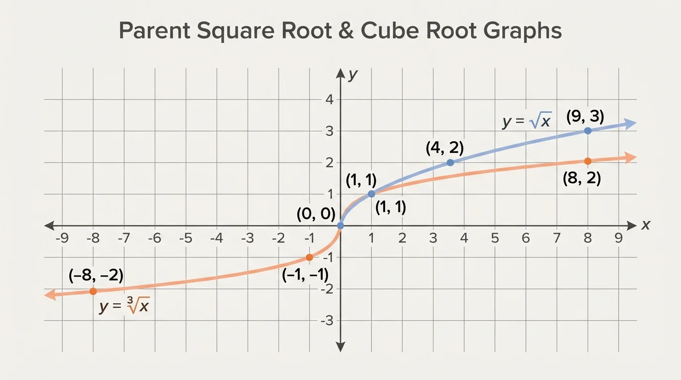
For \(y = \sqrt[3]{x}\), the domain is all real numbers, written \(( -\infty, \infty )\), and the range is also all real numbers. Helpful points are \((-8,-2)\), \((-1,-1)\), \((0,0)\), \((1,1)\), and \((8,2)\). This graph has an S-shaped form, but unlike a cubic function, it becomes steeper near the origin and flatter for larger positive or negative values.
Square root function: a function built from \(\sqrt{x}\) or a transformation of it. Its graph usually has a starting point and extends in one direction.
Cube root function: a function built from \(\sqrt[3]{x}\) or a transformation of it. Its graph usually extends in both directions.
Piecewise-defined function: a function that uses different formulas for different intervals or conditions on \(x\).
A major idea in graphing is that the formula tells you the shape family, while constants and signs tell you how the graph moves. If you can recognize the parent shape, you can often graph the transformed version quickly and accurately.
Transformations, shown in [Figure 2], change the location, orientation, or steepness of a graph. For root functions, it is especially important to track the key starting point or center point. In \(y = \sqrt{x - 3} + 2\), the graph starts at \((3,2)\), not \((0,0)\). The expression \(x - 3\) shifts the graph right by \(3\), and the \( +2\) shifts it up by \(2\).
Here are common transformation patterns:
For square root functions: \[y = a\sqrt{x - h} + k\] The graph starts at \((h,k)\). If \(a > 0\), it extends in the usual direction; if \(a < 0\), it reflects across the x-axis. Larger values of \(\lvert a \rvert\) create a vertical stretch.
For cube root functions: \[y = a\sqrt[3]{x - h} + k\] The graph's central point moves to \((h,k)\). A negative value of \(a\) reflects the graph across the x-axis.
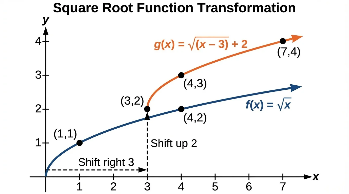
To graph a transformed root function by hand, begin with a few known points from the parent function and move them according to the transformation. For example, for \(y = \sqrt{x - 3} + 2\), take the parent points \((0,0)\), \((1,1)\), \((4,2)\), and \((9,3)\). Shift each point right \(3\) and up \(2\) to get \((3,2)\), \((4,3)\), \((7,4)\), and \((12,5)\).
Later, when you compare different transformed graphs, [Figure 1] still helps because it reminds you what the original parent shape looks like before any shift or reflection happens.
[Figure 3] illustrates the idea behind a piecewise-defined function: a function can follow one rule for some inputs and a different rule for others. Instead of one formula for all \(x\), you read each rule together with its condition.
For example, consider:
\[f(x) = \begin{cases}2x + 1 & \textrm{if } x < 1 \\ x^2 & \textrm{if } x \ge 1\end{cases}\]
To graph this function, graph \(y = 2x + 1\) only for values where \(x < 1\), and graph \(y = x^2\) only where \(x \ge 1\). The boundary point \(x = 1\) matters a lot. Since the first rule uses \(x < 1\), the point from that rule at \(x = 1\) is not included, so you use an open circle. Since the second rule uses \(x \ge 1\), the point from that rule at \(x = 1\) is included, so you use a closed circle.
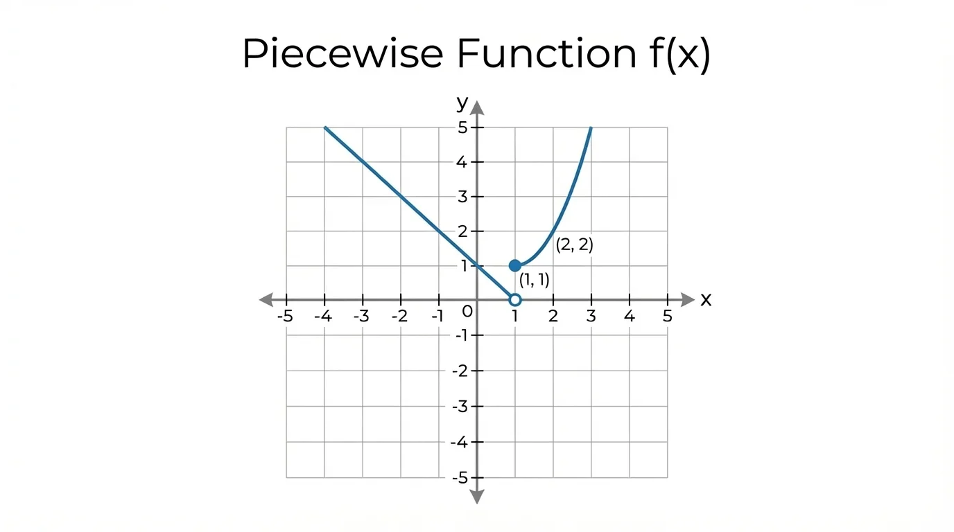
These endpoint symbols prevent one of the most common graphing mistakes: accidentally including a point that should not belong to the graph. An open circle means "not included." A closed circle means "included." If both rules happen to meet at the same point, the graph may look connected, but you still determine inclusion from the inequality symbols.
Piecewise functions are useful because many real systems change behavior after a threshold. A cost plan might charge one rate up to a limit and another rate after that. A machine may operate one way below a certain temperature and another way above it. A graph can show these rule changes clearly.
How to read a piecewise graph
Start by identifying the intervals on which each rule applies. Then graph each formula only on its assigned interval. Finally, check every boundary value and mark the correct endpoint style. A correct graph is not just about plotting the right curve or line; it is also about restricting that graph to the correct part of the coordinate plane.
One strong habit is to test the boundary value in each rule, even if one condition excludes it. This makes it easier to decide where open and closed circles belong and whether the graph has a jump or connects smoothly.
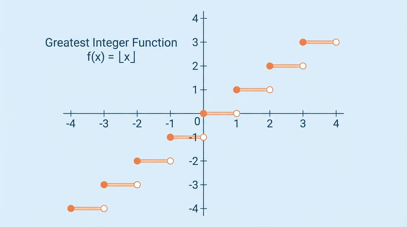
[Figure 4] shows that a step function is a special kind of piecewise function whose graph stays constant on intervals and then jumps. Instead of sloping upward or curving smoothly, the graph forms horizontal "steps." One famous example is the greatest integer function, often written \(f(x) = \lfloor x \rfloor\), which gives the greatest integer less than or equal to \(x\).
For instance, \(\lfloor 2.7 \rfloor = 2\), \(\lfloor -1.2 \rfloor = -2\), and \(\lfloor 5 \rfloor = 5\). On the interval \([2,3)\), the output is always \(2\). That creates a horizontal segment at height \(2\), closed at \(x = 2\) and open at \(x = 3\).
Step functions are important because many everyday quantities change in jumps rather than continuously. Parking garages may charge by each started hour. Shipping prices often stay constant across weight intervals and then jump to a new rate. In digital systems, rounded values also behave like step functions.
When analyzing a step graph, pay attention to where the jumps occur and whether the function is increasing overall, even though it is flat on each separate step. The endpoint markers in [Figure 4] are crucial because they show exactly which input belongs to each horizontal segment.
[Figure 5] shows that the absolute value function is often introduced as distance from zero, but it is also naturally piecewise. Its two-case definition explains why the graph has a sharp V shape instead of a smooth curve.
The definition is:
\[|x| = \begin{cases}x & \textrm{if } x \ge 0 \\ -x & \textrm{if } x < 0\end{cases}\]
For nonnegative values, the output equals the input. For negative values, the output is the opposite of the input, making the result positive. That means \(|3| = 3\) and \(|-3| = 3\).
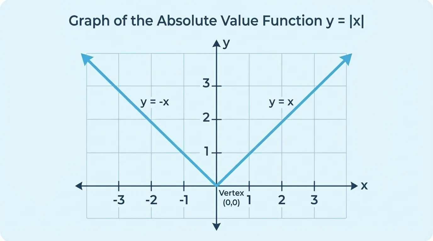
The graph of \(y = |x|\) has vertex \((0,0)\), domain all real numbers, and range \([0,\infty)\). The left branch follows \(y = -x\) for \(x < 0\), and the right branch follows \(y = x\) for \(x \ge 0\). This is a powerful example of a graph made from two linear pieces.
Transformations work here too. For \(y = |x - 2| + 1\), the vertex moves to \((2,1)\). For \(y = -|x| + 4\), the graph reflects across the x-axis and shifts up \(4\), creating an upside-down V.
| Function | Parent Form | Domain | Range | Key Visual Feature |
|---|---|---|---|---|
| Square root | \(y = \sqrt{x}\) | \([0,\infty)\) | \([0,\infty)\) | Starts at one endpoint and increases |
| Cube root | \(y = \sqrt[3]{x}\) | All real numbers | All real numbers | S-shaped graph through the origin |
| Step | \(y = \lfloor x \rfloor\) | All real numbers | Integers | Horizontal steps with jumps |
| Absolute value | \(y = |x|\) | All real numbers | \([0,\infty)\) | V-shaped graph with a vertex |
Table 1. Comparison of major graph families covered in the lesson.
These examples show how symbolic rules turn into graphs with specific features such as endpoints, vertices, and jumps.
Worked example 1: Graph \(y = \sqrt{x + 4} - 1\)
Step 1: Identify the parent function.
The parent is \(y = \sqrt{x}\).
Step 2: Find the transformation.
The expression \(x + 4\) shifts the graph left \(4\), and the \(-1\) shifts it down \(1\).
Step 3: Locate the starting point.
The parent graph starts at \((0,0)\), so the new graph starts at \((-4,-1)\).
Step 4: Generate more points.
Use perfect-square radicands: if \(x + 4 = 0,1,4,9\), then \(x = -4,-3,0,5\). The corresponding points are \((-4,-1)\), \((-3,0)\), \((0,1)\), and \((5,2)\).
The graph begins at \((-4,-1)\) and increases to the right. Its domain is \([ -4, \infty )\), and its range is \([ -1, \infty )\).
This example shows why the starting point matters so much for square root graphs: one quick shift changes both the domain and the visible location of the curve.
Worked example 2: Graph \(y = -2\sqrt[3]{x - 1} + 3\)
Step 1: Identify the parent function.
The parent is \(y = \sqrt[3]{x}\).
Step 2: Describe the transformations.
\(x - 1\) shifts the graph right \(1\). The factor \(-2\) reflects the graph across the x-axis and stretches it vertically by a factor of \(2\). The \( +3\) shifts it up \(3\).
Step 3: Move key parent points.
Parent points \((-8,-2)\), \((-1,-1)\), \((0,0)\), \((1,1)\), and \((8,2)\) become points with \(x\)-values increased by \(1\): \((-7,-2)\), \((0,-1)\), \((1,0)\), \((2,1)\), \((9,2)\).
Step 4: Apply the vertical changes.
Multiply each \(y\)-value by \(-2\) and then add \(3\): \((-7,7)\), \((0,5)\), \((1,3)\), \((2,1)\), and \((9,-1)\).
The graph is a reflected and stretched cube root curve centered around \((1,3)\).
Notice how cube root graphs do not have a starting point the way square root graphs do. Instead, they extend in both directions, so a shifted cube root graph still has all real numbers in its domain.
Worked example 3: Graph the piecewise function
\[g(x) = \begin{cases}-x + 2 & \textrm{if } x < 2 \\ 1 & \textrm{if } x \ge 2\end{cases}\]
Step 1: Graph the first rule on its interval.
Draw the line \(y = -x + 2\) only for \(x < 2\). At \(x = 2\), the line gives \(y = 0\), but since \(x < 2\), plot an open circle at \((2,0)\).
Step 2: Graph the second rule on its interval.
Draw the horizontal line \(y = 1\) only for \(x \ge 2\). Since \(x = 2\) is included, place a closed circle at \((2,1)\).
Step 3: Interpret the graph.
The graph has a jump at \(x = 2\). The left side approaches \(0\), but the function value at \(x = 2\) is \(1\).
This graph combines a decreasing line and a constant piece into one function.
The open and closed circles here work exactly like the endpoint markers in [Figure 3], where the graph switches rules at a boundary value.
Worked example 4: Write \(y = |x - 3|\) as a piecewise function
Step 1: Find where the expression inside the absolute value changes sign.
\(x - 3 = 0\) when \(x = 3\).
Step 2: Use two cases.
If \(x \ge 3\), then \(|x - 3| = x - 3\).
If \(x < 3\), then \(|x - 3| = -(x - 3) = -x + 3\).
Step 3: Write the full piecewise definition.
\[|x - 3| = \begin{cases}-x + 3 & \textrm{if } x < 3 \\ x - 3 & \textrm{if } x \ge 3\end{cases}\]
The graph is a V with vertex at \((3,0)\).
This is one of the clearest examples of how a familiar graph can come directly from two simple linear rules meeting at a vertex.
Root functions appear in measurement, physics, and geometry. For example, if the area of a square is \(A\), then its side length is \(s = \sqrt{A}\). That means the square root graph models how side length changes as area increases. Cube roots appear in volume problems; if a cube has volume \(V\), then its edge length is \(e = \sqrt[3]{V}\).
Piecewise and step functions are even more common in everyday decisions. A mobile data plan may have one pricing rule up to a usage limit and another after that. Tax brackets, postage costs, and hourly billing often behave piecewise. When prices round up to the next hour or next unit, the graph becomes a step function.
Absolute value functions model distance and error. If a sensor is supposed to read \(50\) but instead reads \(x\), then the size of the error is \(|x - 50|\). Engineers and scientists care about the size of the error, not whether it is positive or negative, which is exactly what absolute value represents.
Digital images, sound, and measurements often rely on values being rounded or grouped into intervals. That means step-like behavior appears inside technologies students use every day, even when the graph is hidden behind the screen.
Even the comparison between \(\sqrt{x}\) and \(\sqrt[3]{x}\) has practical meaning. A model with a square root may only make sense for nonnegative quantities such as area or time after a starting moment, while a cube root model can describe signed quantities, including positive and negative changes.
One frequent mistake is forgetting domain restrictions. If you graph \(y = \sqrt{x - 5}\) as though it were defined for all real numbers, the graph will be wrong. Since \(x - 5 \ge 0\), the domain is \(x \ge 5\), so the graph starts at \((5,0)\).
Another mistake is placing open and closed circles incorrectly in piecewise graphs. Always check whether the inequality includes equality. Symbols like \(\le\) and \(\ge\) mean the endpoint is included, so use a closed circle. Symbols like \(<\) and \(>\) mean it is not included, so use an open circle.
A third mistake is transforming the graph in the wrong direction. In \(y = \sqrt{x - 4}\), the graph shifts right \(4\), not left \(4\). A good strategy is to think about the starting point: the radicand becomes zero when \(x = 4\), so the graph must begin there.
For absolute value graphs, students sometimes draw a parabola instead of a V shape. Remember that \(y = |x|\) is built from two lines, not from a quadratic rule. The sharp vertex is one of its defining features, just as [Figure 5] shows.
A reliable graphing checklist is: identify the parent function, find transformations or interval restrictions, determine domain and key points, mark special endpoints or vertices, and then sketch the graph with the correct shape.