A race car can go from nearly at rest to high speed in just a few seconds, while a fully loaded truck takes much longer even with a powerful engine. That difference is not just about "more power" in a vague sense. It reflects a precise pattern in nature: how strongly an object is pushed, how much matter it has, and how quickly its motion changes. Scientists do not accept that pattern just because a textbook states it. They test it by collecting data, organizing it, graphing it, modeling it, and deciding whether the evidence is strong enough to support a claim.
Science depends on evidence that is both valid and reliable. A valid claim is one that is actually supported by the data and by a sensible method of collecting those data. A reliable claim is one that would likely be supported again if the investigation were repeated carefully.
When scientists analyze motion, they are not just measuring how fast something moves. They are often asking a deeper question: What causes the motion to change? To answer that, they use measurements of force, mass, distance, time, and acceleration. Then they look for patterns that hold across many trials, not just one lucky result.
Newton's second law states that the acceleration of an object depends on the net force acting on it and its mass. In mathematical form, it is written as:
\[F_{\textrm{net}} = ma\]
Here, \(F_{\textrm{net}}\) is the net force, \(m\) is the mass, and \(a\) is the acceleration.
That equation is simple, but testing it requires careful data analysis. If the data are messy, incomplete, or poorly measured, the claim may be weak even if the equation is correct. This is why scientists use good tools, repeated trials, and clear mathematical models.
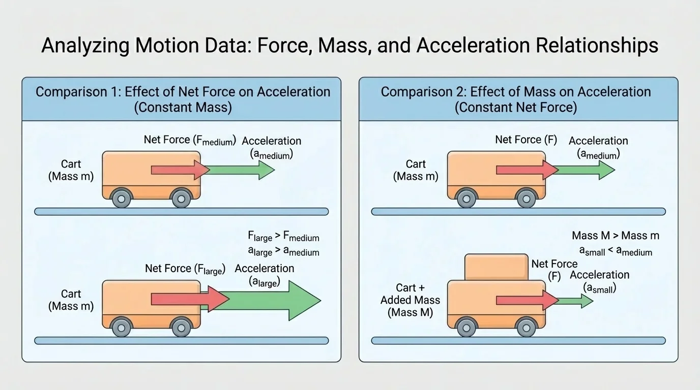
The first step is understanding what each quantity means. Net force is the total force acting on an object after all pushes and pulls are combined, as [Figure 1] illustrates through different force and mass situations. If two students push a cart in opposite directions with equal force, the net force is \(0\), so the cart's motion does not accelerate because of those forces. If one side pushes harder, the cart accelerates in the direction of the larger overall force.
Mass measures how much matter an object has and how strongly it resists changes in motion. Acceleration is the rate at which velocity changes. If a cart speeds up from \(1 \, \textrm{m/s}\) to \(3 \, \textrm{m/s}\) in \(2 \, \textrm{s}\), its acceleration is \(\dfrac{3 - 1}{2} = 1 \, \textrm{m/s}^2\).
Newton's second law connects these quantities:
\[a = \frac{F_{\textrm{net}}}{m}\]
This form shows two key ideas. For a constant mass, increasing net force increases acceleration. For a constant net force, increasing mass decreases acceleration. That is why an empty shopping cart speeds up easily, while a full one feels stubborn.
A numeric example makes the relationship clearer. Suppose a cart has mass \(2 \, \textrm{kg}\) and the net force on it is \(6 \, \textrm{N}\). Then its acceleration is \(a = \dfrac{6}{2} = 3 \, \textrm{m/s}^2\). If the same cart experiences \(10 \, \textrm{N}\), then \(a = \dfrac{10}{2} = 5 \, \textrm{m/s}^2\). If instead the net force stays at \(6 \, \textrm{N}\) but the mass becomes \(3 \, \textrm{kg}\), the acceleration drops to \(a = \dfrac{6}{3} = 2 \, \textrm{m/s}^2\).
Those numbers are not just calculations. They are predictions. A scientific investigation tests whether real data match those predictions closely enough to support the law.
To analyze motion data well, you need both a sound method and the right equipment. A common setup uses a low-friction cart on a track, a force sensor, and a motion sensor. Another setup uses a hanging mass to pull the cart while a digital timer or video-analysis software tracks motion.
Useful tools include motion sensors, photogates, force sensors, digital balances, and video analysis apps. Spreadsheets and graphing software are also important because they help organize trials, calculate acceleration, and generate trend lines. A computational model can simulate how changing force or mass should affect acceleration, allowing scientists to compare predictions with actual measurements.
When you calculate acceleration from motion data, remember that average acceleration can be found from a change in velocity over time: \(a = \dfrac{\Delta v}{\Delta t}\). If you know distance and time for motion starting from rest with nearly constant acceleration, other kinematics relationships can also help estimate acceleration.
A strong investigation controls variables carefully. If you want to test how net force affects acceleration, keep the mass constant. If you want to test how mass affects acceleration, keep the net force constant. If too many variables change at once, the data become difficult to interpret.
Raw measurements often look confusing at first, but clear organization reveals patterns. Scientists usually place data in tables and then create graphs, because [Figure 2] shows how a graph makes proportional trends easier to detect than a list of numbers does. In a force-and-acceleration investigation, the independent variable might be net force, while acceleration is the dependent variable.
Suppose a cart with constant mass \(1.5 \, \textrm{kg}\) is tested under different net forces. The acceleration might be measured from motion sensor data.
| Trial | Net force | Mass | Acceleration |
|---|---|---|---|
| \(1\) | \(1.5 \, \textrm{N}\) | \(1.5 \, \textrm{kg}\) | \(1.0 \, \textrm{m/s}^2\) |
| \(2\) | \(3.0 \, \textrm{N}\) | \(1.5 \, \textrm{kg}\) | \(2.0 \, \textrm{m/s}^2\) |
| \(3\) | \(4.5 \, \textrm{N}\) | \(1.5 \, \textrm{kg}\) | \(3.0 \, \textrm{m/s}^2\) |
| \(4\) | \(6.0 \, \textrm{N}\) | \(1.5 \, \textrm{kg}\) | \(4.0 \, \textrm{m/s}^2\) |
Table 1. Motion data for a cart of constant mass under different net forces.
This table suggests a direct relationship. Each time the net force doubles, the acceleration doubles. Plotting acceleration on the vertical axis and net force on the horizontal axis should produce a straight-line graph through or near the origin if the relationship is proportional.
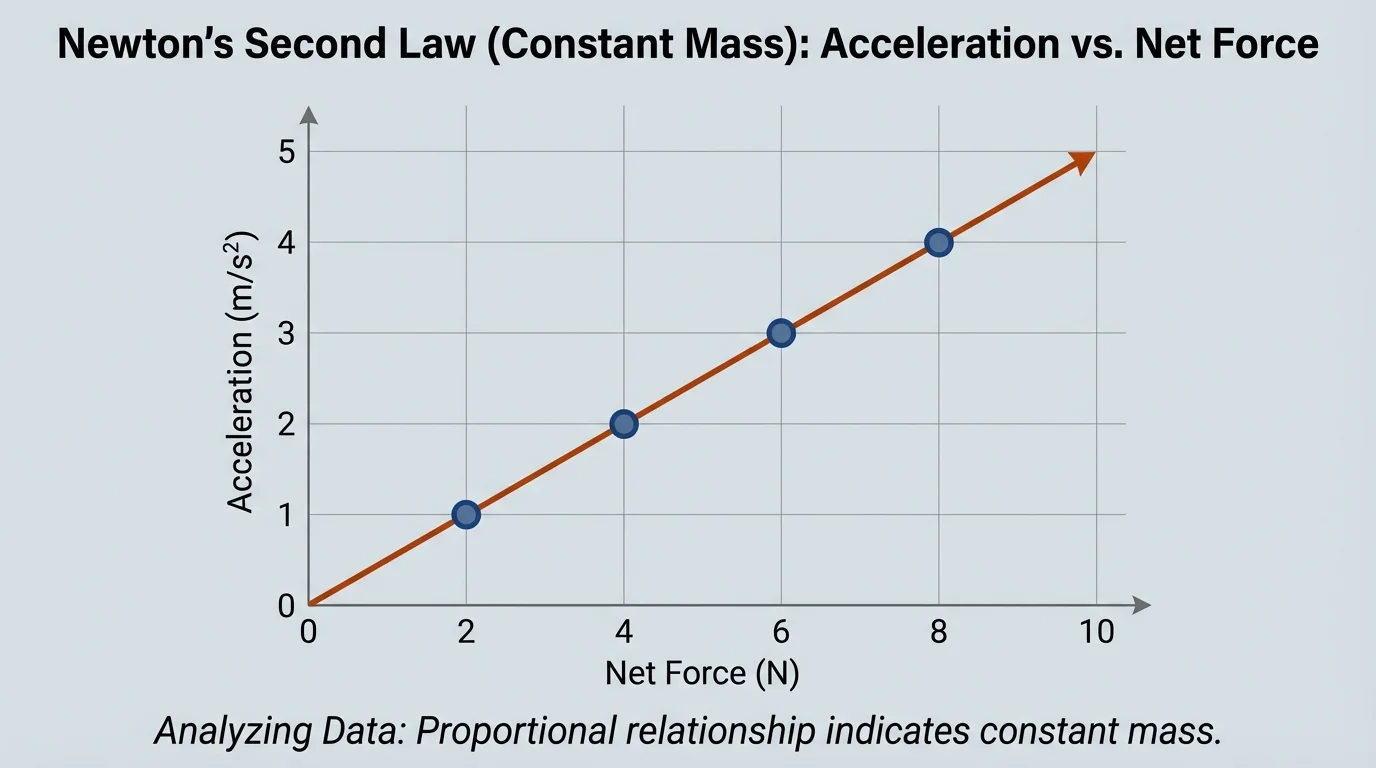
If the graph is nearly linear, that supports the claim that acceleration is directly proportional to net force when mass is constant. The slope of the graph is also meaningful. Since \(a = \dfrac{F_{\textrm{net}}}{m}\), a graph of \(a\) versus \(F_{\textrm{net}}\) has slope \(\dfrac{1}{m}\). For a mass of \(1.5 \, \textrm{kg}\), the slope should be about \(\dfrac{1}{1.5} \approx 0.67\).
Graphs do more than make data look nice. They help you see whether a pattern is linear, curved, scattered, or inconsistent. That matters because the type of pattern affects the claim you can make.
Scientific laws become powerful when they can be expressed as mathematical relationships. A mathematical model describes a system using equations, and [Figure 3] displays how the model changes when mass varies while force stays fixed. In this topic, the model is Newton's second law.
If mass is constant, the model predicts a direct relationship: \(a \propto F_{\textrm{net}}\). If net force is constant, the model predicts an inverse relationship: \(a \propto \dfrac{1}{m}\). That means doubling the mass should cut the acceleration in half, assuming the net force does not change.
Consider a constant net force of \(8 \, \textrm{N}\): if \(m = 1 \, \textrm{kg}\), then \(a = 8 \, \textrm{m/s}^2\). If \(m = 2 \, \textrm{kg}\), then \(a = 4 \, \textrm{m/s}^2\). If \(m = 4 \, \textrm{kg}\), then \(a = 2 \, \textrm{m/s}^2\). The pattern is not linear when plotted as acceleration versus mass; instead, the curve decreases as mass increases.
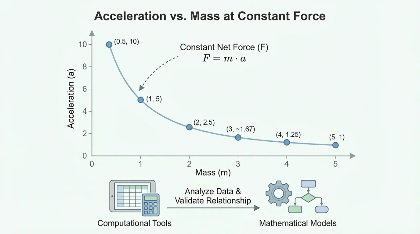
This is where computational tools become especially useful. A spreadsheet can automatically calculate predicted accelerations for many masses or forces. A graphing program can compare measured data points to the model curve. If the data cluster close to the predicted line or curve, confidence in the claim increases.
Engineers use the same kind of data modeling when designing rockets, drones, and electric vehicles. Before a machine is ever built, computer models estimate how changing mass or thrust changes acceleration.
As seen earlier in [Figure 1], the same law explains both why stronger pushes create larger accelerations and why heavier objects respond less. The model does not change from one example to another; only the values do.
Analyzing data means more than reading off numbers. It means deciding what those numbers imply about a claim.
Example 1: Testing force versus acceleration at constant mass
A cart of mass \(2.0 \, \textrm{kg}\) is pulled with different net forces. The measured accelerations are \(1.0 \, \textrm{m/s}^2\), \(2.0 \, \textrm{m/s}^2\), and \(3.0 \, \textrm{m/s}^2\) for net forces of \(2.0 \, \textrm{N}\), \(4.0 \, \textrm{N}\), and \(6.0 \, \textrm{N}\).
Step 1: Compare the ratios \(\dfrac{F_{\textrm{net}}}{a}\).
For trial \(1\): \(\dfrac{2.0}{1.0} = 2.0\). For trial \(2\): \(\dfrac{4.0}{2.0} = 2.0\). For trial \(3\): \(\dfrac{6.0}{3.0} = 2.0\).
Step 2: Interpret the constant ratio.
Because \(\dfrac{F_{\textrm{net}}}{a}\) stays constant at \(2.0\), the data are consistent with \(F_{\textrm{net}} = ma\) for \(m = 2.0 \, \textrm{kg}\).
The data support the claim that acceleration is directly proportional to net force when mass is constant.
One powerful test is to calculate whether the inferred mass from each trial stays the same. If it does, that suggests the data fit the law well.
Example 2: Testing mass versus acceleration at constant force
A net force of \(12 \, \textrm{N}\) acts on three different carts with masses \(2 \, \textrm{kg}\), \(3 \, \textrm{kg}\), and \(6 \, \textrm{kg}\).
Step 1: Use the model \(a = \dfrac{F_{\textrm{net}}}{m}\).
For \(2 \, \textrm{kg}\): \(a = \dfrac{12}{2} = 6 \, \textrm{m/s}^2\).
For \(3 \, \textrm{kg}\): \(a = \dfrac{12}{3} = 4 \, \textrm{m/s}^2\).
For \(6 \, \textrm{kg}\): \(a = \dfrac{12}{6} = 2 \, \textrm{m/s}^2\).
Step 2: Look for the pattern.
When the mass triples from \(2\) to \(6 \, \textrm{kg}\), the acceleration drops from \(6\) to \(2 \, \textrm{m/s}^2\), which is one-third as large.
The data support an inverse relationship between mass and acceleration when net force is constant.
Notice that not every valid conclusion must use exactly the same graph. Some investigations are clearer with a table and ratio check. Others are clearer with a best-fit line or curve.
Example 3: Using measured motion data to infer force
A \(1.8 \, \textrm{kg}\) cart speeds up from \(0.5 \, \textrm{m/s}\) to \(2.9 \, \textrm{m/s}\) in \(3.0 \, \textrm{s}\).
Step 1: Find the acceleration.
\(a = \dfrac{2.9 - 0.5}{3.0} = \dfrac{2.4}{3.0} = 0.8 \, \textrm{m/s}^2\).
Step 2: Use Newton's second law.
\(F_{\textrm{net}} = ma = 1.8 \times 0.8 = 1.44 \, \textrm{N}\).
The motion data imply a net force of \(1.44 \, \textrm{N}\).
These examples show that a scientific claim can come from direct force measurements, from motion measurements, or from a combination of both.
Even when a pattern appears convincing, scientists still ask whether the data quality is strong enough to justify the claim. That is where outliers, repeated trials, and uncertainty matter, and [Figure 4] illustrates how one unusual result can stand apart from a consistent cluster of measurements.
A result may be inaccurate because of friction, miscalibrated sensors, delayed timing, uneven track surfaces, or human reaction time. Some errors are random, causing measurements to scatter above and below the expected value. Others are systematic, shifting many measurements in the same direction.
Suppose five trials for the same setup produce accelerations of \(1.9 \, \textrm{m/s}^2\), \(2.0 \, \textrm{m/s}^2\), \(2.1 \, \textrm{m/s}^2\), \(2.0 \, \textrm{m/s}^2\), and \(3.4 \, \textrm{m/s}^2\). The value \(3.4 \, \textrm{m/s}^2\) is suspicious because it is far from the cluster near \(2.0 \, \textrm{m/s}^2\). It might be an outlier caused by a sensor glitch or recording mistake.
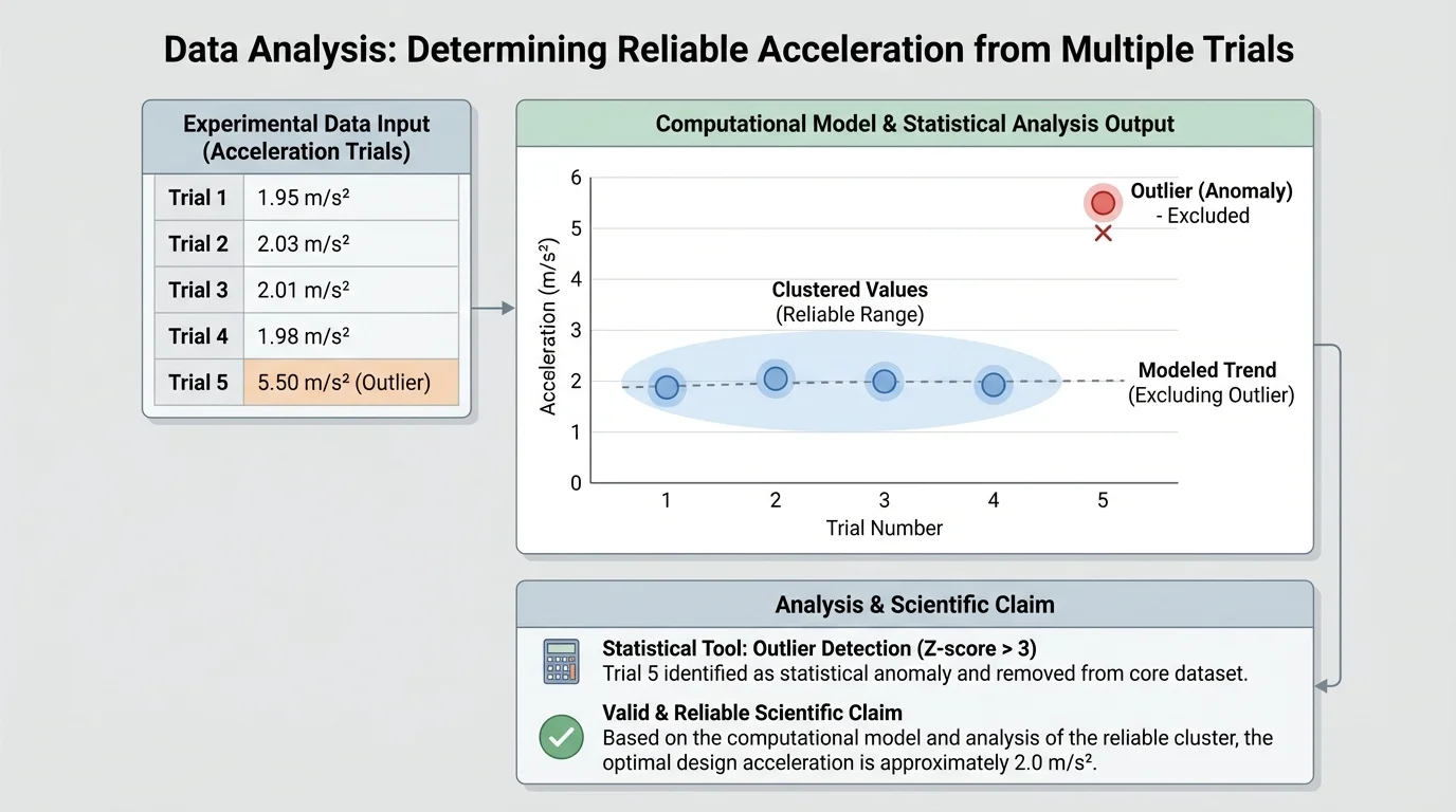
Scientists do not throw out a point just because it is inconvenient. They look for a reason. Was the sensor bumped? Was the force applied differently? Was the trial recorded incorrectly? If there is clear evidence of procedural error, the outlier may be excluded. If not, it must be considered as part of the evidence.
Reliability improves with repeated measurements. If most trials agree closely, confidence rises. If the results vary wildly, the claim is weaker. When the cluster of repeated values matches the mathematical model, as the linear trend in [Figure 2] does for constant mass, that combination of consistency and pattern makes the evidence stronger.
What makes a claim scientifically strong?
A strong scientific claim uses enough data, controls important variables, reports uncertainty honestly, and connects the evidence to a model or principle. It does not depend on a single trial, and it does not ignore data that disagree without explanation.
Validity also depends on whether the method actually tests the claim. For example, if friction changes from trial to trial but is not measured or controlled, then differences in acceleration might not be due only to the intended force change. That would weaken the conclusion.
Analyzing data about force, mass, and acceleration is not only about confirming a law. It also helps solve design problems. Engineers often need to choose an optimal design solution, which means the best design under given constraints such as safety, cost, efficiency, or weight.
In car safety, engineers use crash-test data to understand how forces change the motion of a vehicle and its passengers. They design crumple zones and airbags to reduce acceleration during a collision. Since force is related to acceleration by \(F_{\textrm{net}} = ma\), reducing the acceleration of a passenger reduces the force on the passenger's body.
In robotics, designers compare different motor strengths and robot masses. A heavier robot may be more stable, but it accelerates less for the same motor force. Designers analyze motion data to decide whether the extra stability is worth the slower response. In sports engineering, data help optimize bicycles, running shoes, and protective gear by balancing mass, force transfer, and control.
Design case: choosing between two delivery robots
Robot A has mass \(20 \, \textrm{kg}\) and net driving force \(40 \, \textrm{N}\). Robot B has mass \(25 \, \textrm{kg}\) and net driving force \(55 \, \textrm{N}\).
Step 1: Compute each acceleration.
Robot A: \(a = \dfrac{40}{20} = 2.0 \, \textrm{m/s}^2\).
Robot B: \(a = \dfrac{55}{25} = 2.2 \, \textrm{m/s}^2\).
Step 2: Interpret the result in context.
Robot B accelerates slightly faster, but it is also heavier. If battery life and carrying capacity matter, engineers must consider more than acceleration alone.
The best design depends on the full set of goals and constraints, not just a single number.
That is an important scientific habit: use data to support decisions, but also recognize what your data do and do not measure.
Once data are analyzed, scientists communicate their conclusions using a clear structure: claim, evidence, and reasoning. A claim states what the data support. Evidence includes measurements, graphs, and patterns. Reasoning explains why that evidence supports the claim using accepted scientific ideas.
A strong statement might read like this: The data support the claim that Newton's second law describes the relationship among net force, mass, and acceleration because when mass remained constant, acceleration increased linearly with net force, and when net force remained constant, acceleration decreased as mass increased.
The reasoning part links the data to the law \(F_{\textrm{net}} = ma\). If the data also show repeated, consistent trials with small variation, then the claim is more reliable. If there are large unexplained errors, the claim should be limited or stated more cautiously.
"The important thing is not to stop questioning. Curiosity has its own reason for existing."
— Albert Einstein
Good science is not just getting the "right" answer. It is using tools, technologies, and models to analyze data carefully enough that the answer deserves to be trusted. The same habits that test a physical law also guide real engineering decisions, from safer cars to smarter machines.