Your phone estimates battery life, weather apps predict temperature, and engineers simulate whether a bridge will stay safe in strong wind. None of these predictions comes directly from reality itself. They come from models—carefully designed simplifications of reality. That is both their power and their weakness. A model can tell us a great deal about how a system behaves, but it never includes every detail of the real world. In physics, that limitation matters especially when we track energy, because even small assumptions can change a prediction.
When scientists and engineers build a model, they are not trying to copy the universe in every detail. They are selecting the factors that matter most for a specific question. If the question is how much a cup of coffee cools, the model might focus on thermal energy transfer. If the question is how long a battery can power a speaker, the model might track chemical energy changing into electrical energy and then sound and heat. A model is useful when it captures the main energy changes well enough to make a prediction.
A scientific model is a representation of a system, process, or idea that helps us explain and predict behavior. Models can be physical, mathematical, conceptual, or computational. A globe is a physical model of Earth. A graph of motion is a mathematical model. A computer simulation of a heating system is a computational model.
Models are necessary because real systems are often too large, too small, too fast, too slow, or too complicated to study directly in every detail. You cannot track every molecule in a car engine or every air current around a building. Instead, you make reasonable approximations. This lets you calculate likely outcomes, test ideas, and compare predictions to measurements.
Model means a simplified representation of a real system used to explain or predict behavior.
Prediction is a result produced by a model about what will happen under certain conditions.
Approximation is a value or description that is close to, but not exactly equal to, the real one.
Assumption is something the model treats as true in order to make analysis possible.
The key idea is not that a model is "right" in some absolute sense. The key idea is that a model is useful within limits. A simple model may be excellent for one purpose and poor for another. For example, treating a moving car as a single object works well when predicting its kinetic energy, but it fails if you want to know how heat spreads through the engine parts.
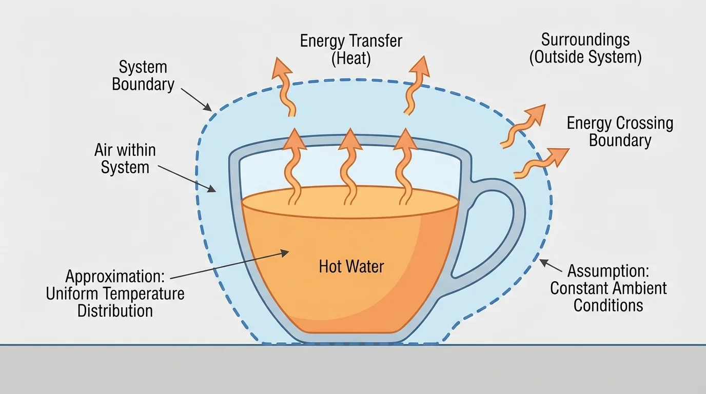
[Figure 1] To use energy models well, you first need to define a system. In physics, a system is the part of the world you choose to study. Everything else is the surroundings. The boundary between them matters because energy can be transferred across that boundary by heating, mechanical work, radiation, electricity, or moving matter.
A system may contain one component or several components. For example, in a hot drink cooling on a desk, one component could be the liquid and another could be the surrounding air. In a flashlight, one component is the battery and another is the bulb. In each case, energy can shift between components and also flow into or out of the entire system.
When we track energy, we are using the idea of conservation of energy. Energy is not created or destroyed. It is transferred between parts of a system or transformed from one form to another. That makes energy accounting possible. If one component loses energy, something else must gain energy, or the energy must leave the system.
This is why scientists often talk about the change in energy of a component rather than just "how much energy it has." A change in energy compares a final state to an initial state. If a component warms up, speeds up, rises higher, or stores more elastic energy, its energy change is positive. If it cools down, slows down, or releases stored energy, its energy change is negative.
From earlier physics work, remember that energy can appear in different forms, including kinetic, gravitational potential, elastic, thermal, chemical, electrical, and radiant energy. A useful model may track only the forms that matter most for the question being asked.
Choosing the system correctly is one of the most important modeling decisions. If you choose a battery alone as the system, electrical energy leaving the battery counts as energy flowing out. If you choose the battery and bulb together as the system, that same transfer is now internal to the system. The equations are still valid, but the bookkeeping changes.
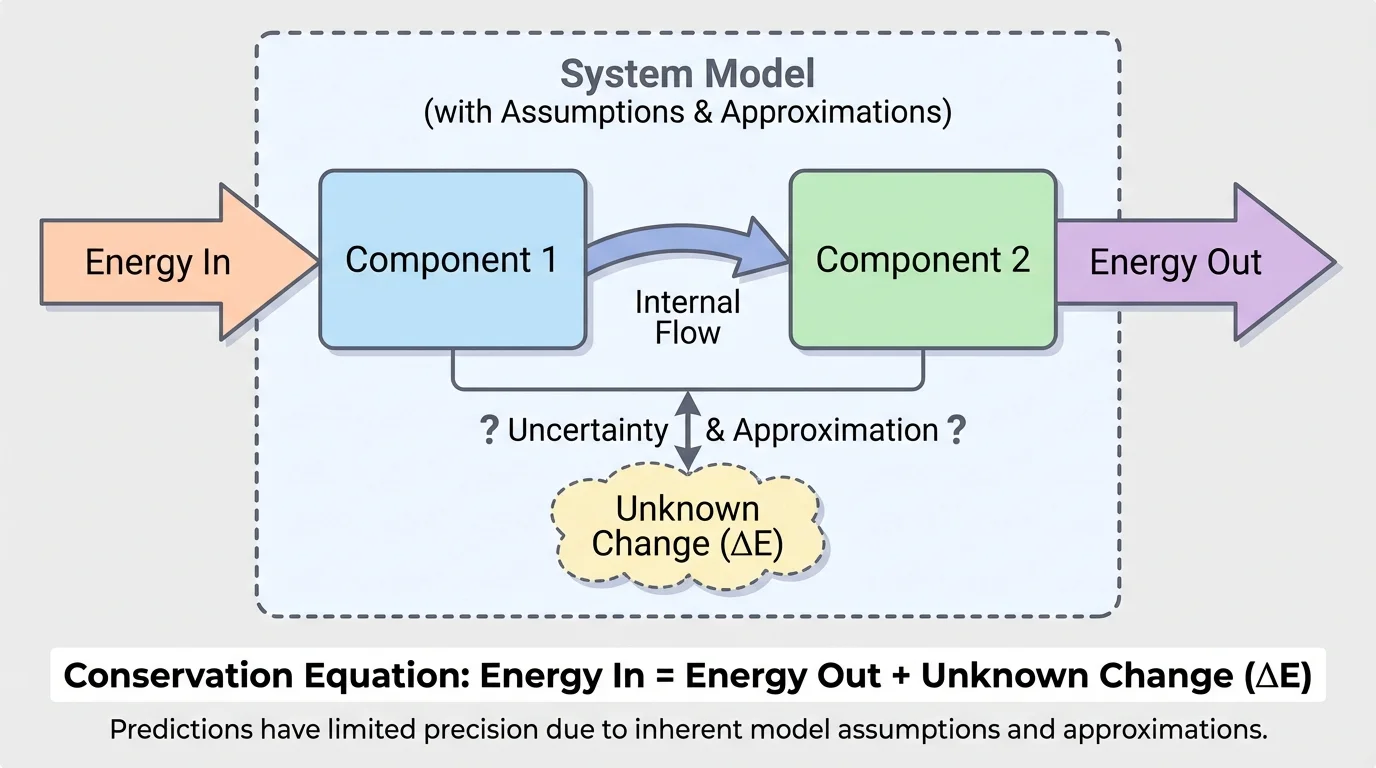
[Figure 2] A computational model uses rules, equations, and known values to calculate unknown quantities. For energy in systems, one of the simplest and most powerful rules is an energy-balance equation. The model tracks changes in the energy of components along with energy entering and leaving the system.
If a system has two components, labeled component 1 and component 2, a useful relationship is
\[\Delta E_1 + \Delta E_2 = E_{in} - E_{out}\]
Here, \(\Delta E_1\) and \(\Delta E_2\) are the changes in energy of the two components. The quantity \(E_{in}\) is the energy transferred into the system, and \(E_{out}\) is the energy transferred out of the system. If you know three of these quantities, you can solve for the fourth.
To calculate the change in energy of one component, rearrange the equation. For example, if you want to solve for the change in energy of component 1, then
\[\Delta E_1 = E_{in} - E_{out} - \Delta E_2\]
This is a model because it simplifies the situation into measurable quantities. It assumes that all important energy changes are included in the terms. If some energy transfer is ignored, the prediction will be off.
In many grade-level physics problems, this model is enough to make strong predictions. But notice what it does not tell you by itself. It does not guarantee that you measured every transfer correctly. It does not guarantee that no energy escaped in an untracked form such as sound or unwanted heating. The equation is exact as a law of physics, but the model built from measured and selected terms can still be incomplete.
Why computational models are powerful
A computational model can repeat calculations quickly, compare many scenarios, and reveal patterns that are hard to see by inspection. For example, a computer can test how changing insulation thickness affects the thermal energy loss of a house over many hours. But every output depends on the assumptions entered at the start. Better code does not remove bad assumptions.
A good habit is to ask two questions every time you use an energy model: What am I including? and What am I leaving out? Those questions often matter more than the arithmetic.
Now consider how the model works in concrete situations. These examples show that the calculations can be straightforward even though the interpretation requires care.
Example 1: Battery and motor
A toy car system includes a battery and a motor. During a short interval, the motor gains \(18 \textrm{ J}\) of energy, and \(5 \textrm{ J}\) of energy leaves the system as sound and heating to the surroundings. No energy enters the system from outside. Find the change in energy of the battery.
Step 1: Write the energy-balance equation.
Use \(\Delta E_{battery} + \Delta E_{motor} = E_{in} - E_{out}\).
Step 2: Substitute known values.
Here, \(\Delta E_{motor} = 18 \textrm{ J}\), \(E_{in} = 0 \textrm{ J}\), and \(E_{out} = 5 \textrm{ J}\). So \(\Delta E_{battery} + 18 = 0 - 5\).
Step 3: Solve.
\(\Delta E_{battery} = -5 - 18 = -23 \textrm{ J}\).
The battery's energy change is \(-23 \textrm{ J}\). The negative sign means the battery lost energy.
This result makes physical sense. The battery supplies energy to the motor, and some energy also leaves the system as sound and heat. The model is simple, but it captures the major transfers.
Example 2: Hot metal in cooler water
A system contains a hot metal block and cooler water in an insulated container. The water gains \(120 \textrm{ J}\) of thermal energy. The container is not perfectly insulated, and \(15 \textrm{ J}\) leaves the system to the surroundings. No energy enters from outside. Find the change in energy of the metal block.
Step 1: Set up the equation.
\(\Delta E_{metal} + \Delta E_{water} = E_{in} - E_{out}\).
Step 2: Substitute values.
\(\Delta E_{metal} + 120 = 0 - 15\).
Step 3: Solve for the metal block.
\(\Delta E_{metal} = -15 - 120 = -135 \textrm{ J}\).
The metal block loses \(135 \textrm{ J}\) of energy.
Notice how the answer is larger in magnitude than the water's gain alone. That is because the metal transfers energy both to the water and to the surroundings. If a student ignored the \(15 \textrm{ J}\) leaving the system, the model would predict \(-120 \textrm{ J}\) instead of \(-135 \textrm{ J}\).
Example 3: Falling object with air resistance
A ball and Earth are treated as a system. As the ball falls, the system's gravitational potential energy decreases by \(50 \textrm{ J}\). During the fall, \(8 \textrm{ J}\) leaves the system as thermal energy to the surrounding air because of drag. Find the change in kinetic energy of the system.
Step 1: Identify the two energy changes being tracked.
Let \(\Delta E_k\) be the change in kinetic energy and \(\Delta E_g = -50 \textrm{ J}\) be the change in gravitational potential energy.
Step 2: Write the balance.
\(\Delta E_k + \Delta E_g = E_{in} - E_{out}\).
Step 3: Substitute and solve.
\(\Delta E_k - 50 = 0 - 8\), so \(\Delta E_k = 42 \textrm{ J}\).
The kinetic energy increases by \(42 \textrm{ J}\).
This example shows something important about models. In a simplified "no air resistance" model, the kinetic energy increase would be \(50 \textrm{ J}\). In a more realistic model, some energy leaves to the air, so the prediction becomes \(42 \textrm{ J}\). Both models use conservation of energy, but they include different assumptions.
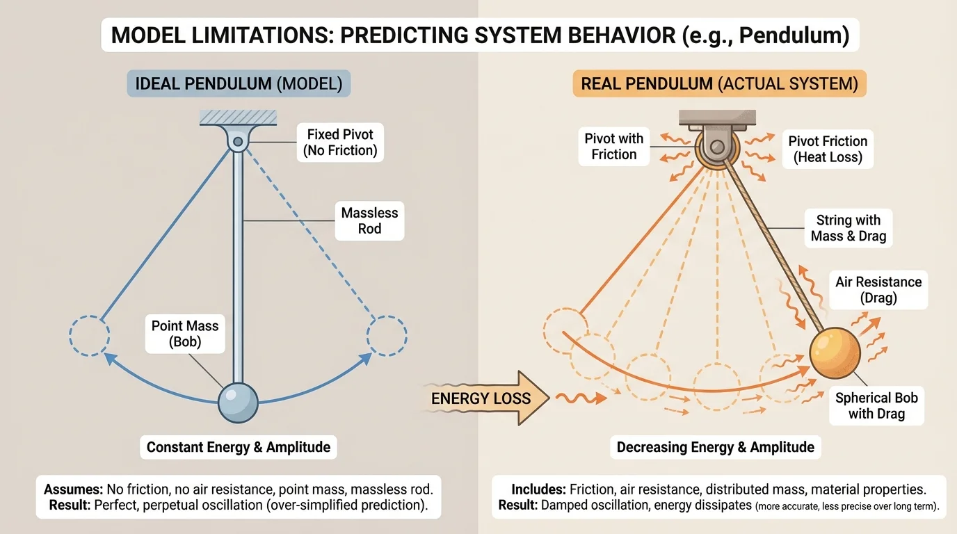
[Figure 3] Every model leaves something out. That is not a mistake; it is a design choice. The challenge is deciding whether the ignored details are small enough to neglect. In mechanical systems, for example, a model may ignore friction or air resistance. In thermal systems, it may assume perfect insulation. In electrical systems, it may treat wires as having no resistance. An ideal model can be elegant while still missing real energy losses.
Assumptions often make calculations possible. If you assume a room is perfectly insulated, then no energy leaves or enters, so \(E_{in} = 0\) and \(E_{out} = 0\). That simplifies the model dramatically. But actual rooms are never perfectly insulated. Heat leaks through walls, windows, and air gaps. The prediction may still be useful over a short time, but it becomes less reliable over a longer time.
Another common approximation is treating variables as constant when they really change. A model might assume a constant rate of energy transfer, even though that rate slows as temperatures become more equal. It might assume constant friction, even though surfaces warm up and change. These choices can be reasonable first approximations, but they limit precision.
Measurement also introduces assumptions. Suppose sensors report values to the nearest \(1 \textrm{ J}\). Then a calculated energy change cannot honestly claim precision smaller than the measurements support. If your inputs are approximate, your output will also be approximate.
Weather forecasting depends on extremely advanced models, yet even with satellites, radar, and supercomputers, forecasts become less reliable further into the future. Tiny uncertainties in starting conditions grow over time, which is a powerful reminder that better models still have limits.
Sometimes a model is limited because the system itself is complex. Biological systems, ecosystems, climate systems, and real machines involve many interacting parts. Tracking all energy pathways may be impossible in practice. Scientists then choose the pathways most likely to matter and test whether the model matches observations.
Precision describes how exact or finely resolved a value is. Reliability describes how much trust we should place in a model's prediction. A model might produce a number like \(42.783 \textrm{ J}\), but that does not mean the real system behaved with that exact value. If the assumptions are rough and the measurements are uncertain, writing many decimal places can create a false sense of certainty.
A useful way to think about this is that every prediction has two parts: the calculation and the confidence you have in that calculation. The arithmetic may be correct while the model is still incomplete. For instance, if a student forgets to include sound energy leaving a speaker system, the computed answer may be mathematically correct for the incomplete model but physically inaccurate for the real situation.
There are several common sources of limited precision and reliability:
The pendulum example from [Figure 3] makes this visible. An ideal pendulum model predicts repeated motion with no loss of mechanical energy. A real pendulum gradually slows because energy is transferred to the surroundings by air resistance and friction at the pivot. The simple model is still valuable for understanding the main motion, but it is not perfectly reliable for long-term prediction.
| Model Feature | Simple Model | More Realistic Model | Effect on Prediction |
|---|---|---|---|
| Friction | Ignored | Included | Lower mechanical energy over time |
| Insulation | Perfect | Imperfect | Energy can leave the system |
| Transfer rate | Constant | Variable | Prediction changes with time |
| Measurements | Exact values assumed | Uncertain values used | Output has uncertainty |
Table 1. Comparison of common simplifying assumptions and how they affect energy-model predictions.
Scientists improve models by comparing predictions to observations, identifying mismatches, and then refining the assumptions. If a cooling model predicts that a drink reaches room temperature in \(10 \textrm{ min}\) but measurements show \(14 \textrm{ min}\), that difference gives information. Maybe the model treated heat transfer as constant when it actually slowed over time. Maybe the cup material mattered more than expected.
Refining a model often means adding one important factor at a time. In a falling-object model, you might first ignore air resistance, then include a simple drag term, then include changes in air density. Each new version may improve reliability, but it also increases complexity. There is always a trade-off between simplicity and realism.
"All models are wrong, but some are useful."
— George Box
This famous statement does not mean models are failures. It means models are selective. They are tools, not perfect copies of reality. A model can be excellent for making one kind of prediction and poor for another. For many physics tasks, the best model is the simplest one that captures the important energy changes accurately enough.
Even the system-boundary idea from [Figure 1] helps improve models. By redefining the system, you can sometimes reduce uncertainty. If energy transfers between two objects are hard to measure separately, choosing both objects as one system may simplify the accounting.
Energy models are used throughout science and engineering. In building design, engineers model how energy enters and leaves a house through sunlight, heating systems, walls, and ventilation. These predictions help reduce energy waste. In electronics, designers estimate how much electrical energy becomes useful output and how much becomes unwanted thermal energy. In medicine, thermal models help understand how quickly body tissue heats or cools during treatment.
Sports science also uses energy models. When analyzing a runner, scientists may track chemical energy from food, kinetic energy of motion, and thermal energy released to the surroundings. The model will not capture every muscle fiber and every microscopic transfer, but it can still predict performance trends and energy demands.
Environmental science depends heavily on large-scale energy modeling. Earth's climate involves incoming solar energy, outgoing infrared radiation, ocean heat storage, cloud effects, and many feedback loops. These models are far more complex than a classroom example, yet they still rely on the same central idea: track energy changes and transfers carefully, then test predictions against data.
Case study: Laptop battery heating
A laptop battery loses \(300 \textrm{ J}\) of chemical energy during a short interval. Of that, \(220 \textrm{ J}\) is transferred electrically to the computer's components, and \(55 \textrm{ J}\) leaves the battery directly as thermal energy to the surroundings. Determine whether the energy accounting balances if these are the only significant transfers.
Step 1: Interpret the known values.
The battery's energy change is \(\Delta E = -300 \textrm{ J}\). Energy leaving electrically and thermally accounts for \(220 + 55 = 275 \textrm{ J}\).
Step 2: Compare model and reality.
The difference is \(300 - 275 = 25 \textrm{ J}\).
Step 3: Explain the result.
If the model assumed only those two output pathways, then \(25 \textrm{ J}\) is unaccounted for. That suggests either measurement uncertainty or an additional transfer path inside the system, such as temporary internal heating.
This is how models are used in practice: not just to compute, but to reveal what may be missing.
That last example is especially realistic. In real engineering, a model that fails to balance perfectly is not always discarded. Instead, scientists ask whether the mismatch is within measurement uncertainty or whether the model needs revision.
Good scientific thinking does not treat a model's output as unquestionable truth. It treats the output as a prediction with conditions attached. A careful scientist states the assumptions, identifies the likely sources of uncertainty, and explains the range in which the prediction is expected to work.
That means answers should be interpreted in context. If a simple energy model predicts \(42 \textrm{ J}\), the important question is not only "What number did I get?" but also "How reliable is that number?" Was friction ignored? Were measurements rounded? Was the system boundary chosen well? Were all major energy flows tracked in the computational model from [Figure 2]?
In physics, the most powerful models are often the ones that are simple enough to use and honest enough about their limits. They help us calculate unknown energy changes, reveal patterns in systems, and make practical decisions. At the same time, they remind us that prediction is never the same thing as certainty.