A mountain range can look permanent when you drive past it, yet over millions of years it rises, cracks, and erodes. A bridge can appear solid and unchanging, yet in a fraction of a second it can fail if forces exceed its design limits. Science often begins with this surprising truth: some systems seem stable only because we are observing them on the wrong time scale. To understand the world well, we must study not only what changes, but also how fast, why, and whether the change can be undone.
In both natural systems and human-built systems, conditions of stability and the factors that determine rates of change are central to understanding how systems behave. A forest, a city water supply, the human body, a battery, a coastline, and the global climate are all systems. Each contains parts that interact. Each can remain relatively stable for a time. Each can also shift, sometimes gradually and sometimes suddenly.
A system is a set of connected parts that influence one another. In science, systems can be as small as a single cell or as large as Earth's climate. Engineers also study systems: power grids, roads, buildings, airplanes, and communication networks. A system is considered stable when its key features stay within certain limits, even if small changes happen inside it.
Stability does not mean "nothing happens." Your body temperature stays near a narrow range even though heat is constantly produced and lost. A building remains standing even though wind, vibration, and temperature changes act on it every day. Stability means the system resists disturbance or returns to a balanced condition after disturbance.
Stability is the tendency of a system to remain within a certain range of conditions or to return to that range after a disturbance.
Rate of change is how much a quantity changes in a certain amount of time.
Irreversible change is a change that cannot naturally or practically be returned to its original state.
When scientists ask whether a system is stable, they also ask what could change it and how quickly that change might happen. This is why the study of change is closely connected to prediction. If a system is changing slowly, people may have time to respond. If the rate of change is extremely high, action may need to be immediate.
Many systems are dynamic rather than static. That means they are always undergoing processes, even when they appear steady. A lake may maintain a similar water level because inflow and outflow are nearly balanced. A city may keep its electrical supply stable because operators constantly adjust generation to match demand. Stability often depends on balance among competing processes.
Some systems reach equilibrium, a condition in which opposing processes balance one another. Equilibrium does not always mean complete stillness. In chemistry, reactions can continue in both directions while overall concentrations remain constant. In ecosystems, births and deaths may continue while total population size changes little.
However, stability has limits. If rainfall drops too much, a lake may shrink. If electrical demand suddenly spikes, a power grid may become unstable. These examples show that systems often stay stable only under certain conditions. Once a threshold is crossed, the rate of change can increase sharply.
Some of the most dramatic changes in nature begin with long periods of apparent calm. Stress can build up slowly along a fault line for years, then be released in seconds during an earthquake.
This is one reason scientists pay close attention to both present conditions and trends over time. A system that looks safe right now may be moving toward a critical point.
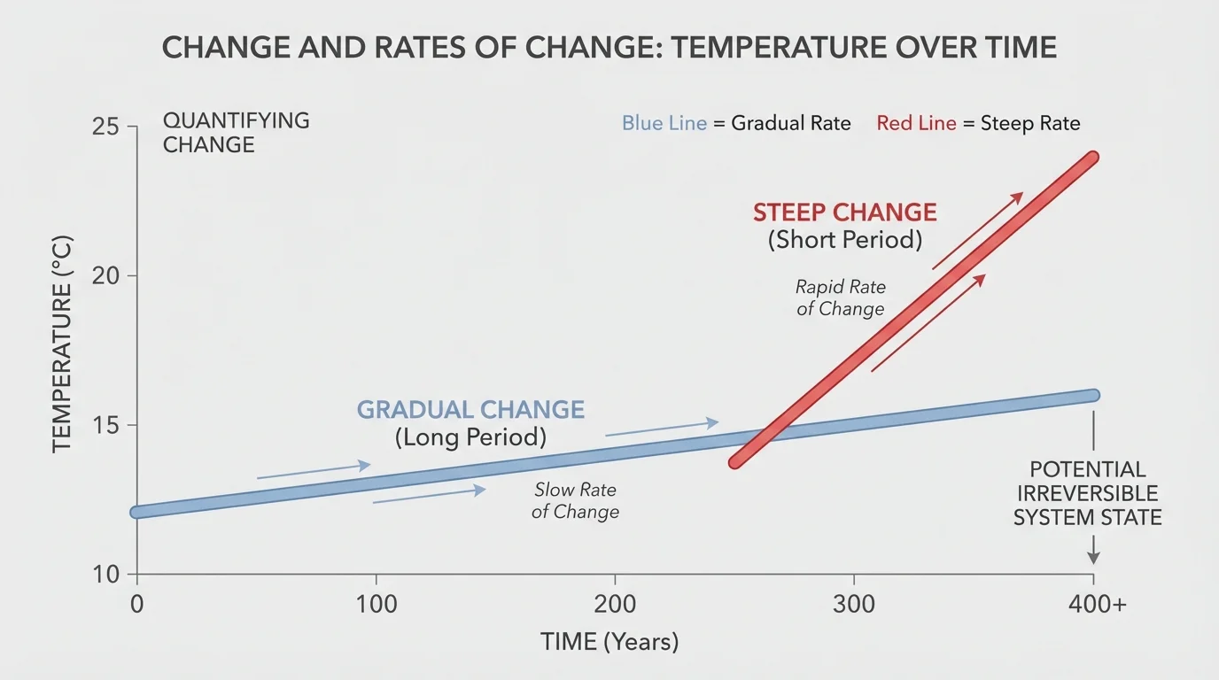
To study change scientifically, we need measurement. A variable is any quantity that can change, such as temperature, speed, population, mass, or concentration. The basic idea of rate is simple: compare how much the variable changes to how much time passes. [Figure 1] illustrates this relationship on a graph, where steeper lines represent faster change.
The average rate of change is calculated by dividing the change in a quantity by the change in time:
\[\textrm{average rate of change} = \frac{\textrm{change in quantity}}{\textrm{change in time}}\]
If a plant grows from \(12 \textrm{ cm}\) to \(20 \textrm{ cm}\) in \(4 \textrm{ days}\), the average rate of growth is \(\dfrac{20 - 12}{4} = \dfrac{8}{4} = 2 \textrm{ cm/day}\). This does not mean the plant grew exactly \(2 \textrm{ cm}\) each day. It means that, on average, this was the overall pace of change.
Units matter. Speed may be measured in \(\textrm{m/s}\), population growth in organisms per year, cooling in \(^\circ\textrm{C}/\textrm{min}\), and erosion in millimeters per century. Choosing the right unit helps reveal whether a change is fast or slow.
Rate can also be positive, negative, or zero. If temperature rises, the rate is positive. If battery charge decreases, the rate is negative. If the quantity stays constant over the interval measured, the rate is zero. A graph with a horizontal line shows no change over time.
Numeric example: calculating average rate of change
A reservoir holds \(500{,}000 \textrm{ L}\) of water on Monday and \(470{,}000 \textrm{ L}\) on Thursday. Find the average rate of change over \(3\) days.
Step 1: Find the change in quantity.
The reservoir changes by \(470{,}000 - 500{,}000 = -30{,}000 \textrm{ L}\).
Step 2: Divide by the change in time.
\(\dfrac{-30{,}000 \textrm{ L}}{3 \textrm{ days}} = -10{,}000 \textrm{ L/day}\).
The negative sign means the water level is decreasing at an average rate of \(10{,}000 \textrm{ L/day}\).
As we saw with line steepness, the same total change can occur over different time intervals, producing very different rates. Losing \(30{,}000 \textrm{ L}\) in \(3\) days is far more serious than losing that amount in \(3\) months.
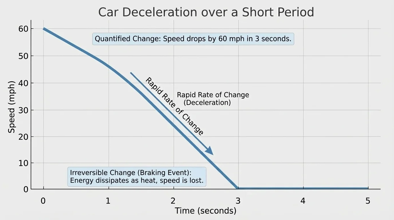
Some changes happen so quickly that even a few seconds matter. In a car crash, speed, momentum, and force change in fractions of a second. In the human body, electrical signals in the heart occur in milliseconds. In chemistry, some reactions happen almost instantly once conditions are right. Rapid change is especially important because people may have little time to respond, as [Figure 2] makes clear with a sharp drop in speed during braking.
Suppose a car slows from \(24 \textrm{ m/s}\) to \(0 \textrm{ m/s}\) in \(3 \textrm{ s}\). Its average rate of change of speed is \(\dfrac{0 - 24}{3} = -8 \textrm{ m/s}^2\). The negative value indicates the speed is decreasing. In physics, this is negative acceleration.
Short time scales are also important in natural hazards. During an earthquake, strain may build for decades but ground motion occurs in seconds. During a flash flood, river level can rise rapidly after intense rainfall. The speed of the change, not just the final amount, determines how dangerous the event is.
Fast changes can also occur in biology. Blood glucose may rise quickly after a meal and then fall as hormones regulate it. Nerve impulses travel rapidly along neurons. Medical monitoring devices must often measure change second by second because average values over long intervals can hide urgent problems.
Engineers designing airbags, earthquake-resistant buildings, or emergency cooling systems care deeply about short-term rates of change. A material or device that handles slow change may fail under sudden stress.
Other changes are too slow to notice directly in a single day or even a single lifetime. Coastlines shift through erosion, mountains wear down, species evolve, and climates change over decades to millennia. A slow rate does not make a change unimportant. In fact, slow changes can become enormous when enough time passes.
If a cliff erodes at an average rate of \(2 \textrm{ mm/year}\), that seems tiny. But over \(500\) years, the total retreat is \(2 \times 500 = 1{,}000 \textrm{ mm} = 1 \textrm{ m}\). This is a good reminder that long time scales can turn small yearly changes into major transformations.
Long-term rates are central in climate science. Global average temperature may change by only fractions of a degree in a decade, yet that shift can alter storms, drought patterns, sea level, and ecosystems. Similarly, structures such as bridges, pipelines, and dams degrade slowly through corrosion, fatigue, or weathering. If these trends are ignored, failure becomes more likely later.
Time scale changes what we notice. A system may look stable on one time scale and unstable on another. A forest appears steady from week to week, but over decades it may change due to wildfire frequency, invasive species, rainfall shifts, and human land use. Scientists choose time scales carefully so they do not miss important patterns.
The same principle applies to human populations, disease spread, and resource use. A city can grow at what seems like a modest annual rate, yet over several decades the demand for water, food, housing, and transportation can increase dramatically.
Measurements tell us what has happened; models help us understand why it happens and predict what may happen next. Scientists and engineers build models using graphs, equations, computer simulations, and physical prototypes. Different systems follow different patterns of change, and these patterns are easier to recognize when graphed, as [Figure 3] illustrates.
One common pattern is linear change, in which a quantity changes by roughly the same amount in equal time intervals. If a tank loses \(5 \textrm{ L}\) each minute, the relationship is approximately linear.
Another pattern is exponential change, in which the amount of change depends on how much is already present. Populations of bacteria under ideal conditions can grow this way. Money in a compound-interest account also follows exponential growth. At first the curve may look gentle, but it can become very steep.
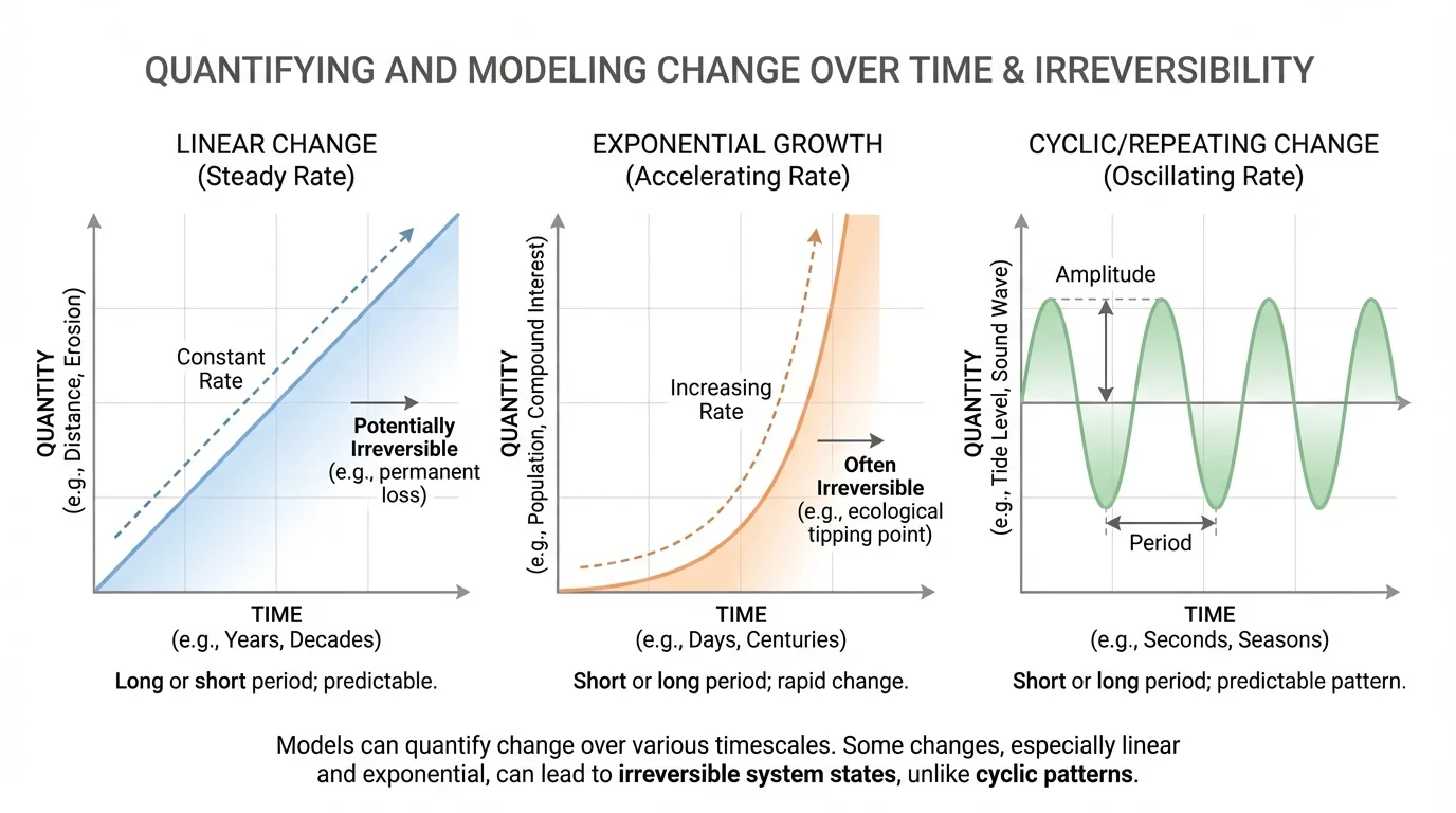
A third pattern is cyclic change, in which changes repeat. Day and night, the seasons, tides, and some economic patterns are cyclic. Not all systems follow just one pattern; some may switch from one type to another when conditions change.
Models are simplifications. They do not include every detail, but a good model captures the most important relationships. For example, a cooling object can often be modeled by tracking how the temperature difference between the object and its surroundings changes over time. Epidemiologists use models to estimate how infections spread. Climate scientists use models to simulate interactions among atmosphere, ocean, land, and ice.
Comparing the curves in [Figure 3] helps explain why prediction can be difficult. A system that has been changing slowly may suddenly accelerate if it follows an exponential trend or if a threshold is crossed.
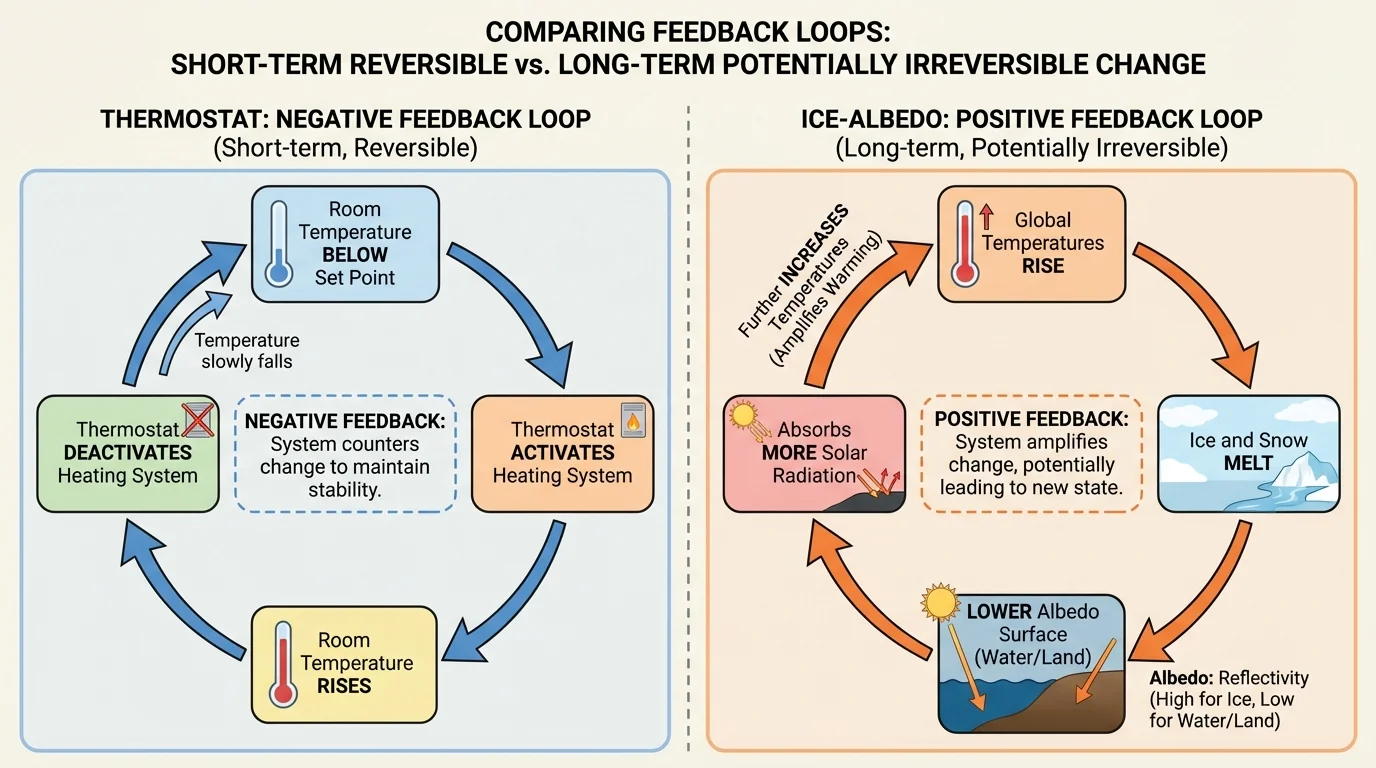
Many systems remain stable because of feedback loops. A feedback loop occurs when a system's output influences its own future behavior. These loops can either reduce change or amplify it, as [Figure 4] shows by contrasting two very different examples.
Negative feedback reduces departures from a desired state. A thermostat is a classic example. If room temperature drops below the set point, the heater turns on. As the room warms, the heater turns off. This keeps the temperature within a relatively stable range. In the body, sweating and shivering help regulate temperature in a similar way.
Positive feedback amplifies change. One climate example involves ice and sunlight. Ice reflects a large fraction of incoming sunlight. If ice melts, darker ocean or land is exposed and absorbs more energy, causing more warming and more melting. This is a positive feedback because the initial change reinforces itself.
Some systems are resilient, meaning they can absorb disturbances and still function. Others are fragile and may shift into a new state after a tipping point. A lake can remain clear for years, but if nutrient input rises too far, algae growth may suddenly increase and the water may become cloudy and oxygen-poor. Returning to the original state may be difficult even if the original cause is reduced.
From earlier science study, recall that causes and effects in systems are rarely isolated. A change in one part of a system often triggers additional changes elsewhere. Feedback is one of the main reasons system behavior can become complex.
This is why scientists do not only measure current conditions. They also monitor indicators that suggest whether a system is approaching a critical threshold.
Not all changes are alike. Some can be undone relatively easily; others cannot. A change is reversible change if the system can return to its earlier state, at least approximately. It is irreversible if returning is impossible or so difficult that it is not practical. [Figure 5] compares these types of change directly. This distinction is essential when evaluating environmental damage, resource use, and engineering safety.
Melting ice is often reversible because cooling can freeze the water again. Stretching a spring slightly may also be reversible if the spring returns to its original shape. But burning wood is a different kind of change. Combustion creates new substances such as \(\textrm{CO}_2\), water vapor, ash, and heat. The original piece of wood cannot simply be restored by cooling it.
Rusting is another common example. When iron reacts with oxygen and moisture, it forms iron oxides. This chemical change is generally irreversible in everyday conditions. Similarly, once an egg is cooked, the proteins have changed structure in ways that are not easily reversed.
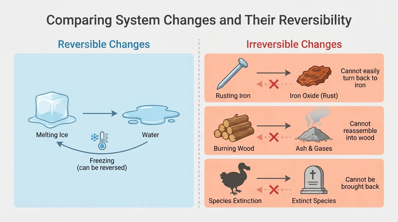
Some irreversible changes occur in ecosystems and societies. Species extinction is effectively irreversible on human time scales. Groundwater depletion, loss of fertile topsoil, and contamination by long-lasting pollutants can also be extremely difficult to undo. These examples matter because prevention is often far easier than repair.
Chemical example: irreversible combustion
When methane burns in oxygen, the reaction is
\[\textrm{CH}_4 + 2\textrm{O}_2 \rightarrow \textrm{CO}_2 + 2\textrm{H}_2\textrm{O}\]
The reactants and products are different substances. Even though matter is conserved, the original methane and oxygen are no longer present in the same form. This is why combustion is treated as an irreversible change in ordinary conditions.
The comparison also reminds us that reversibility is sometimes a matter of scale and practicality. In theory, some changes can be reversed with enough energy and technology. In practice, the cost or difficulty may make them effectively irreversible.
In medicine, rates of change can matter more than single measurements. A slowly rising temperature may suggest one problem, while a rapid drop in blood pressure may signal an emergency. In environmental science, the rate at which glaciers lose mass helps researchers estimate future water supply and sea-level rise. In engineering, the rate of crack growth in a bridge or aircraft component helps determine inspection schedules and maintenance needs.
City planners also use rate-of-change data. If a population is growing by \(3\%\) per year, schools, roads, hospitals, and water systems must expand accordingly. If rainfall patterns change over decades, drainage systems may need redesign. A built system that was stable under past conditions may become unstable under new ones.
Economies show similar patterns. Prices, employment, and production can change gradually or suddenly. A small yearly inflation rate can noticeably affect costs over time. A rapid market crash can alter behavior in hours. Although economic systems differ from physical systems, the same idea applies: understanding rates of change helps people prepare and respond.
Engineers sometimes design structures not just for the maximum force they may face, but for how quickly that force may be applied. A material can withstand a heavy load added slowly yet fail if the same load is delivered suddenly.
Across all these examples, one lesson stands out: measuring only the amount of change is not enough. The rate, pattern, and reversibility of change are equally important.
A single system can show several kinds of change at once. Earth's climate includes daily weather fluctuations, seasonal cycles, and long-term warming trends. A forest may experience rapid change during a wildfire, medium-term regrowth over years, and slow soil formation over centuries. A bridge may vibrate in milliseconds, expand and contract with daily temperature changes, and slowly corrode over decades.
That is why scientists ask multiple questions: What is changing? How much is it changing? Over what time interval? What factors control the rate? Is the system stable, or only temporarily stable? Is the change reversible, or is action needed before a point of no return is reached?
Understanding stability and change gives us a more realistic view of the world. It teaches us that calm does not always mean safety, slow does not always mean harmless, and rapid does not always mean random. With careful measurement, good models, and attention to feedback and irreversibility, we can better understand both natural processes and the systems we build.