A single gene can influence a trait in one organism, but when that trait is tracked across hundreds or thousands of organisms, patterns begin to appear. Those patterns are not just biological observations; they are mathematical ones. Scientists use algebra to ask questions such as: if the probability of inheriting a trait is known, what distribution should appear in a population? If a bacterial population doubles instead of adding a fixed number each hour, how fast will it grow? These questions matter in genetics, medicine, agriculture, and ecology.
Biology often looks messy because living things vary, but that variation does not mean there is no pattern. In heredity, scientists study how traits are passed from parents to offspring and how those traits are distributed in populations. Algebra helps organize those patterns by representing quantities as variables and showing how one quantity changes when another changes.
For example, a scientist may track the frequency of a certain expressed trait over generations. If the proportion changes steadily, a linear model may describe the pattern. If the proportion grows by repeated multiplication, an exponential model may work better. The goal is not only to describe what happened, but also to predict what may happen next.
From earlier math work, remember that a variable stands for a quantity that can change. A relationship between variables can be shown with words, a table, a graph, or an equation. In science, these forms represent real measurements, not just abstract numbers.
When scientists build models, they are simplifying reality. A model can be useful even when it is not perfect. In genetics, for instance, a probability model may predict an expected ratio such as \(\dfrac{3}{4}\) and \(\dfrac{1}{4}\), but actual data from a real population may differ because of chance, environmental effects, mutation, or limited sample size.
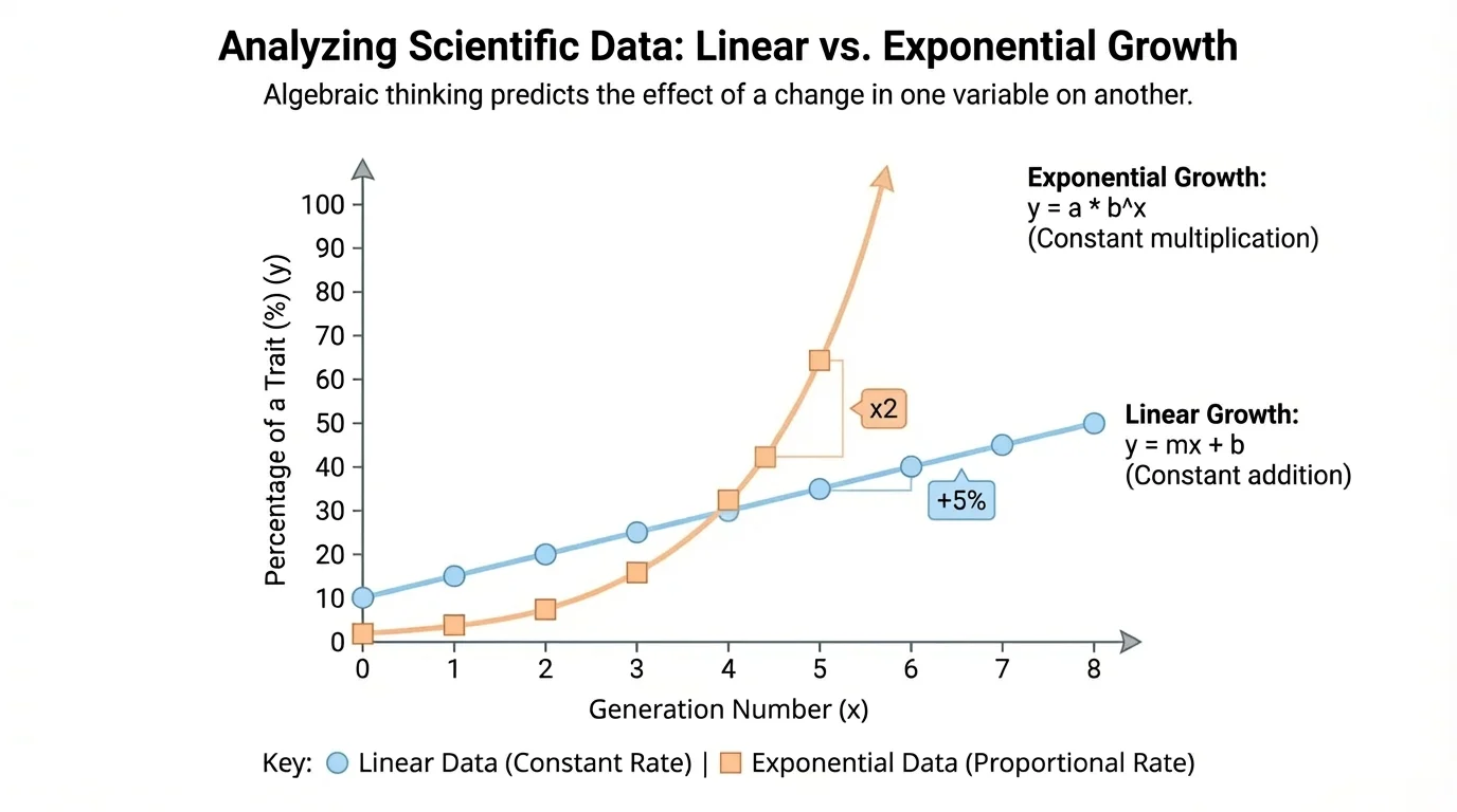
[Figure 1] In scientific investigations, the independent variable is the quantity that is changed or selected, while the dependent variable is the quantity that responds. In a heredity study, generation number might be the independent variable, while the percentage of individuals showing a trait might be the dependent variable. Scientists often plot these relationships on graphs because a visual pattern can reveal whether the relationship is steady, curved, scattered, or unpredictable.
Biological data nearly always include variation. If a trait such as height is measured in a population, not every individual will have the same value. Instead, the data form a distribution. Some traits cluster around an average, while others appear in distinct categories, such as attached versus unattached earlobes. Understanding the shape of the distribution helps scientists decide what kind of model makes sense.
Suppose a population of flowering plants is studied for purple petals. In generation \(1\), \(40\%\) show purple petals. In generation \(2\), \(44\%\) show purple petals. In generation \(3\), \(48\%\) show purple petals. This suggests a steady increase of \(4\) percentage points per generation. A simple linear model would be useful here because the change from one generation to the next is constant.
Linear relationship means one variable changes by a constant amount when another variable changes by equal intervals.
Exponential relationship means one variable changes by a constant factor, not a constant amount, when another variable changes by equal intervals.
Probability is the likelihood that an event will occur, usually written as a number from \(0\) to \(1\), a fraction, or a percent.
Those definitions matter because many biology questions ask which type of change is taking place. A constant increase of \(5\) organisms each day is very different from growth that multiplies by \(2\) each day. At first, the numbers may look similar, but after several intervals the difference becomes dramatic.
Inheritance is often described with probability because offspring do not all receive identical combinations of alleles. If two heterozygous parents for a trait with dominant-recessive inheritance are crossed, the expected genotype ratio is \(1:2:1\), and the expected phenotype ratio is often \(3:1\). Algebra helps connect these ratios to actual population counts.
If \(p\) is the probability that one offspring shows a dominant phenotype, and \(n\) is the total number of offspring, then the expected number with that phenotype is
\(E = pn\)
If \(p = \dfrac{3}{4}\) and \(n = 200\), then
\[E = \frac{3}{4} \cdot 200 = 150\]
So the expected number of offspring showing the dominant phenotype is \(150\). The expected number showing the recessive phenotype is \(200 - 150 = 50\).
Trait distribution example
A class studies a fast-growing plant species. From a cross, the probability of tall plants is \(\dfrac{3}{4}\), and the probability of short plants is \(\dfrac{1}{4}\). There are \(120\) offspring.
Step 1: Find the expected number of tall plants.
Tall plants: \(\dfrac{3}{4} \cdot 120 = 90\)
Step 2: Find the expected number of short plants.
Short plants: \(\dfrac{1}{4} \cdot 120 = 30\)
Step 3: Interpret the result.
If inheritance follows the expected probability closely, the distribution should be near \(90\) tall and \(30\) short, although the exact counts may differ in real life.
The algebra gives an expectation, not a guarantee.
That last point is essential. Probability predicts what tends to happen over many events. In a very small sample, random chance can cause noticeable deviations. If only \(4\) offspring are observed, getting exactly \(3\) dominant and \(1\) recessive is possible, but not certain. In a sample of \(400\), the observed distribution usually comes closer to the expected ratio.
This is where statistics becomes important. Scientists compare observed data to expected values and ask whether the difference is small enough to be explained by chance or large enough to suggest another factor is involved.
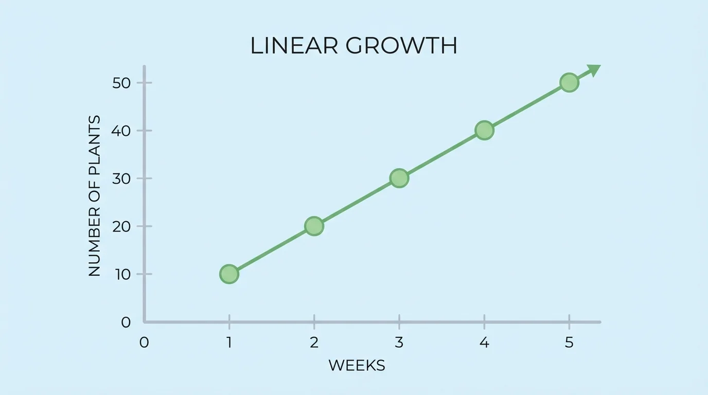
[Figure 2] A linear growth pattern occurs when a quantity increases by the same amount in equal intervals. In biology, this can describe situations such as a laboratory population that receives a fixed number of new individuals every week, or a measured trait that changes at a roughly constant rate. The graph of linear growth is a straight line because equal horizontal steps produce equal vertical changes.
The general algebraic form of a linear relationship is
\(y = mx + b\)
Here, \(m\) is the rate of change, also called the slope, and \(b\) is the starting value when \(x = 0\).
Suppose a scientist starts with \(20\) seedlings and adds \(5\) new seedlings to the study each week. If \(w\) is the number of weeks and \(S\) is the number of seedlings, then
\(S = 5w + 20\)
After \(6\) weeks, the number of seedlings is
\[S = 5(6) + 20 = 50\]
One way to recognize linear growth is to look for a constant difference in a table.
| Week | Seedlings | Change |
|---|---|---|
| \(0\) | \(20\) | — |
| \(1\) | \(25\) | \(+5\) |
| \(2\) | \(30\) | \(+5\) |
| \(3\) | \(35\) | \(+5\) |
| \(4\) | \(40\) | \(+5\) |
Table 1. A linear pattern with a constant increase of \(5\) seedlings per week.
If the difference between consecutive outputs remains constant, a linear model is a strong candidate. This kind of algebraic thinking lets a scientist extend the pattern and predict future values without measuring every single week.
Some biological quantities look linear only over a limited interval. A teenager's height, for example, may increase at a nearly constant rate for a period of time even though growth over the entire lifespan is not linear.
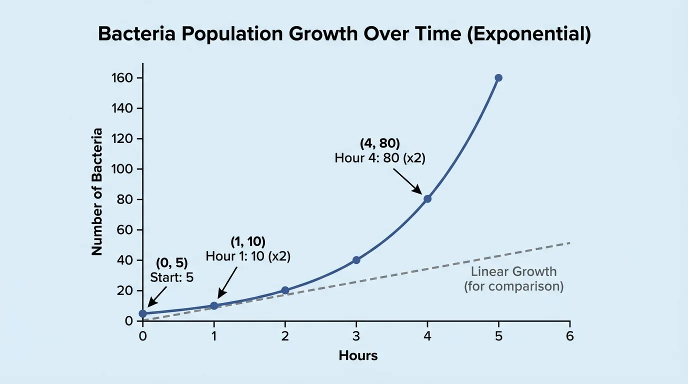
[Figure 3] Exponential growth occurs when a quantity is multiplied by the same factor in equal intervals. This is common in biology when cells divide, bacteria reproduce, or a population grows without major environmental limits. The curve rises slowly at first and then steeply, which is a classic sign of repeated multiplication rather than repeated addition.
The general form of exponential growth is
\(y = a(b)^x\)
In this equation, \(a\) is the starting amount and \(b\) is the growth factor. If \(b > 1\), the quantity increases exponentially.
Suppose a bacterial culture starts with \(100\) bacteria and doubles every hour. If \(t\) is time in hours, then the population \(P\) is modeled by
\[P = 100(2)^t\]
After \(4\) hours,
\[P = 100(2)^4 = 100 \cdot 16 = 1{,}600\]
Unlike linear growth, exponential growth has a constant ratio between outputs. In the bacteria example, each hour's population is \(2\) times the previous hour's population.
| Hour | Bacteria | Ratio |
|---|---|---|
| \(0\) | \(100\) | — |
| \(1\) | \(200\) | \(\times 2\) |
| \(2\) | \(400\) | \(\times 2\) |
| \(3\) | \(800\) | \(\times 2\) |
| \(4\) | \(1{,}600\) | \(\times 2\) |
Table 2. An exponential pattern with a constant growth factor of \(2\).
Cell division example
A single cell divides into \(2\) cells every cycle. How many cells are present after \(6\) cycles if the process starts with \(1\) cell?
Step 1: Write an exponential model.
Starting amount \(a = 1\), growth factor \(b = 2\), number of cycles \(x = 6\).
So \(N = 1(2)^x\).
Step 2: Substitute \(x = 6\).
\(N = 1(2)^6 = 64\)
Step 3: Interpret.
After \(6\) cycles, there are \(64\) cells. The number increases rapidly because each cycle multiplies the previous total.
This is why exponential patterns can become very large in surprisingly little time.
Real populations do not grow exponentially forever. Food, space, predators, disease, and waste buildup eventually limit growth. Even so, exponential models are extremely useful for short time periods or ideal laboratory conditions.
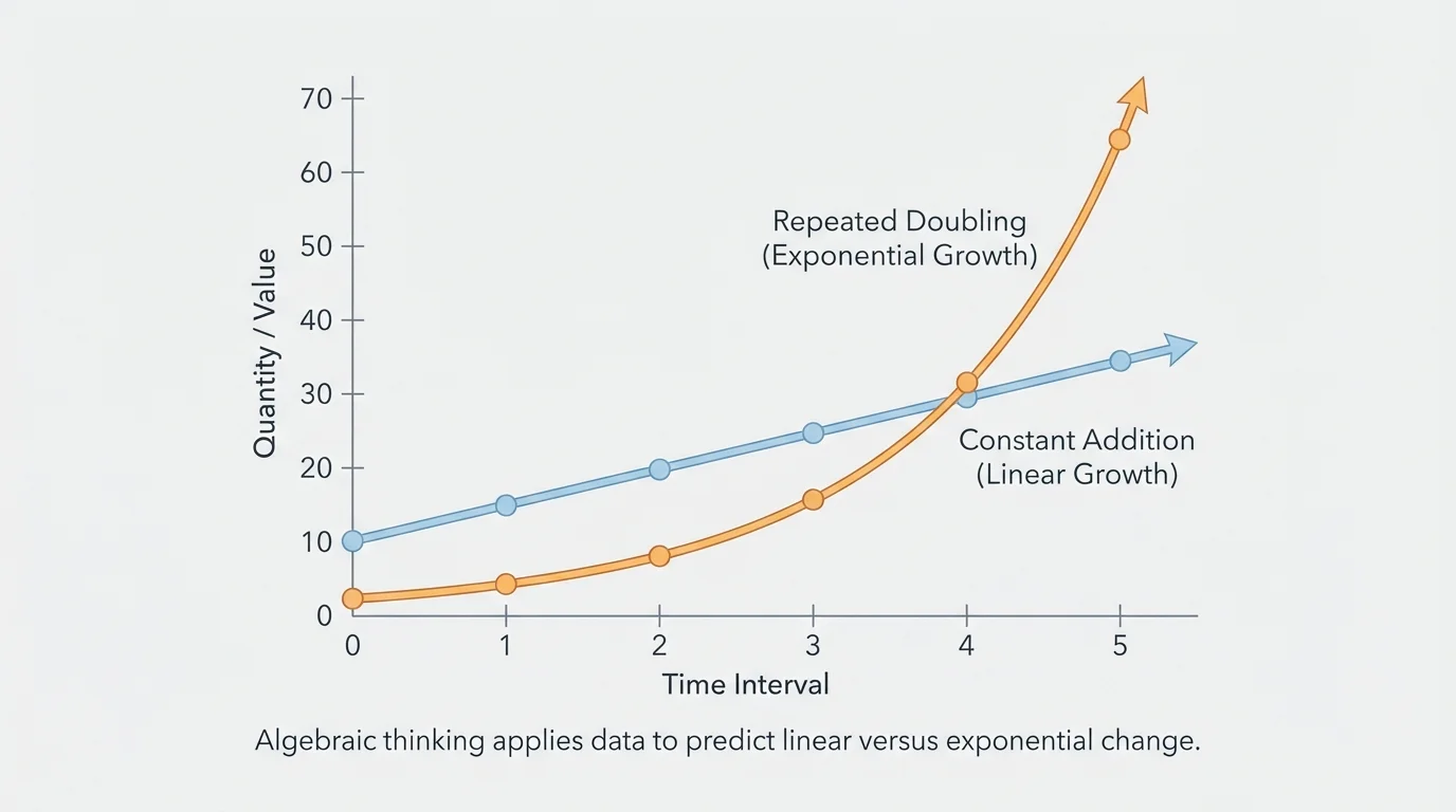
[Figure 4] At a glance, linear and exponential data can both look like "growth," but they behave very differently. The figure compares the two on the same axes, making the contrast clear: linear change adds the same amount each interval, while exponential change multiplies by the same factor.
Consider two populations that both start at \(10\). Population A grows linearly by \(10\) each day, so its model is \(A = 10d + 10\). Population B doubles each day, so its model is \(B = 10(2)^d\).
On day \(1\), both are \(20\). On day \(2\), both are \(40\). But on day \(3\), population A is \(40\) while population B is \(80\). By day \(6\), population A is \(70\), but population B is \(640\). Early on, the patterns may seem similar; later, the difference becomes enormous.
This distinction matters in genetics and population biology. A trait spreading through a population might appear to rise slowly at first, then quickly. That pattern can signal multiplicative change, such as when each generation of carriers produces more carriers. By contrast, a fixed increase in observed cases per year suggests a linear trend.
As we saw earlier in [Figure 2] and [Figure 3], the quickest way to tell the difference is to examine differences and ratios. Constant difference suggests linearity. Constant ratio suggests exponential change.
Why graphs matter for biological interpretation
A table of numbers is useful, but a graph can reveal structure faster. A straight line suggests a constant rate of change. A curve that gets steeper suggests multiplicative growth. In real biological data, points may not sit exactly on a perfect line or curve, so scientists look for the overall pattern rather than expecting exact matches.
Algebraic thinking also helps scientists move from simple offspring probabilities to population-level predictions. If \(p\) is the probability of a trait appearing and \(n\) is the total number of individuals, then the expected count is \(pn\). If a trait appears in \(30\%\) of a population of \(500\), the expected number is
\[0.30 \cdot 500 = 150\]
So about \(150\) individuals are expected to show that trait.
Suppose researchers track a recessive trait in a population of insects over time. If the number of individuals expressing the trait rises by \(12\) each generation, a linear model may fit. If the number rises by a factor of \(1.5\) each generation, an exponential model may fit better. These models help biologists forecast future distributions and test whether a pattern is likely due to inheritance alone or influenced by environmental pressures.
Population prediction example
A recessive trait appears in \(18\%\) of a population of \(250\) organisms. Estimate the number expressing the trait. Then suppose the population grows to \(400\) while the percentage stays the same.
Step 1: Convert the percent to a decimal.
\(18\% = 0.18\)
Step 2: Find the expected count in \(250\).
\(0.18 \cdot 250 = 45\)
Step 3: Find the expected count in \(400\).
\(0.18 \cdot 400 = 72\)
The expected count increases from \(45\) to \(72\) because the population size changes even though the trait frequency stays constant.
Notice that a change in one variable does not always mean the same kind of change in another. If population size increases while trait percentage stays constant, the count of individuals with the trait changes proportionally. If both the population size and the trait frequency change, the relationship becomes more complex and may require a more detailed model.
No model captures every detail of life. A genetic probability model assumes that inheritance follows a certain pattern and that many offspring are observed. Real data may differ because populations are small, mating is not random, environmental factors affect survival, or new mutations appear.
For example, if a trait is expected in \(25\) out of \(100\) offspring but only \(19\) are observed, that does not automatically mean the model is wrong. Chance alone can cause some deviation. However, if the difference is consistently large across repeated trials, scientists may suspect that another variable is influencing the outcome.
This is why biology relies on both algebra and statistics. Algebra provides a model of how variables relate. Statistics evaluates how well the model matches the evidence. Together, they allow scientists to reason carefully from data instead of guessing from isolated observations.
"The purpose of a model is not to capture every detail, but to reveal the pattern that matters."
In medicine, genetic counselors use probabilities to discuss the chance that offspring may inherit certain conditions. They do not promise exact outcomes for one family; instead, they use population-based probabilities and known inheritance patterns to estimate risk.
In agriculture, plant and animal breeders track trait frequencies across generations. If a desirable trait rises at a steady rate, a linear model may describe the trend over a limited period. If selective breeding causes rapid multiplication of a trait in a controlled population, the pattern may look more exponential.
In conservation biology, scientists monitor populations that carry rare alleles. They ask how population size, reproduction rate, and environmental pressure may affect the future distribution of those alleles. The same algebraic reasoning used in a classroom table can help guide decisions about habitat protection and breeding programs.
In microbiology, the difference between linear and exponential growth can be the difference between a manageable infection and a dangerous outbreak. A bacterial population that doubles repeatedly can reach huge numbers far sooner than intuition suggests, as the steep curve discussed earlier makes clear.