A change of just \(1\%\) may sound tiny, but when it happens again and again, the result can become dramatic. That is why a savings account, a viral video, a shrinking population of bacteria under treatment, and the value of a used car can all be modeled with the same kind of function: an exponential function. The key is learning how to read the expression carefully, especially when it is written in a form that hides the rate or the time scale.
An exponential function models situations where a quantity changes by the same percent over equal intervals of time. This is different from linear change, where the same amount is added or subtracted each time. In exponential change, the quantity is multiplied by the same factor over and over.
For example, if a quantity increases by \(2\%\) each year, then each year it becomes \(1.02\) times as large as before. If it decreases by \(3\%\) each year, then each year it becomes \(0.97\) times as large as before. Those multipliers, \(1.02\) and \(0.97\), are what reveal the percent rate of change.
Percent increase and percent decrease from earlier algebra are essential here. A percent increase of \(r\) means multiply by \(1+r\) when \(r\) is written as a decimal. A percent decrease of \(r\) means multiply by \(1-r\).
If the percent is \(5\%\), write it as the decimal \(0.05\). Then an increase gives the factor \(1.05\), while a decrease gives the factor \(0.95\). This simple idea is the foundation for interpreting every exponential expression in this lesson.
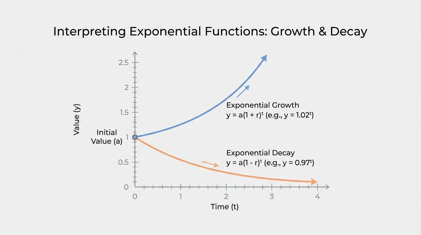
[Figure 1] A common form of an exponential model is \(y=a(b)^t\). Here, \(a\) is the initial value, meaning the value when \(t=0\), and \(b\) is the growth or decay factor. When the base \(b\) is greater than \(1\), the graph rises, and when \(0<b<1\), the graph falls.
The number \(b\) tells how the quantity changes during one time unit. If \(b=1.08\), the function grows by \(8\%\) each time unit. If \(b=0.92\), the function decays by \(8\%\) each time unit, because \(1-0.92=0.08\).
There are two fast interpretation rules:
If \(b>1\), the function represents exponential growth.
If \(0<b<1\), the function represents exponential decay.
Initial value is the starting amount, found when \(t=0\).
Growth factor is the multiplier used for each time unit when the quantity increases.
Decay factor is the multiplier used for each time unit when the quantity decreases.
Percent rate of change is the percent increase or decrease in one time unit, found from the factor.
To move between factor and percent, use these relationships:
For growth, \(b=1+r\), so \(r=b-1\).
For decay, \(b=1-r\), so \(r=1-b\).
Here, \(r\) is the decimal form of the percent rate. To write it as a percent, multiply by \(100\).
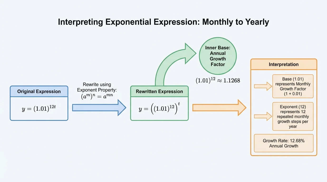
[Figure 2] Sometimes an exponential function is written in a form that hides the rate per larger time unit. The equivalent forms come from exponent rules, and those forms often make interpretation easier. Rewriting a function can reveal whether a rate is happening monthly, yearly, or over some other interval.
The main exponent property we use is
\[a^{mn}=(a^m)^n\]
This means that \((1.01)^{12t}\) can be rewritten as \(((1.01)^{12})^t\). That new form shows what happens in one year if \(t\) measures years and there are \(12\) monthly changes each year.
Another useful property is
\[a^{t/n}=(a^{1/n})^t\]
So \((1.2)^{t/10}\) can be rewritten as \(((1.2)^{1/10})^t\). This shows that the quantity grows by the factor \((1.2)^{1/10}\) for each single time unit if the original \(1.2\) factor applies over a span of \(10\) time units.
Why rewriting matters
Two exponential expressions can represent the same function while emphasizing different features. One form may highlight the number of repeated steps, while another reveals the percent rate for one larger interval. Interpreting functions often means choosing the form that makes the important property easiest to see.
When you rewrite a function, you are not changing the relationship. You are only changing how clearly it communicates the behavior of the function.
The classification depends on the factor being applied over the relevant interval. If the factor is greater than \(1\), the quantity grows. If it is between \(0\) and \(1\), the quantity decays. This is true whether the expression is simple, like \((1.02)^t\), or rewritten, like \(((1.01)^{12})^t\).
Be careful: the exponent may change the time scale, but it does not change the basic idea. You still look for the multiplier associated with one complete interval of the variable you are using.
Now we apply these ideas to the kinds of functions you are expected to interpret.
Worked example 1
Interpret \(y=(1.02)^t\).
Step 1: Identify the factor.
The base is \(1.02\).
Step 2: Decide whether it represents growth or decay.
Since \(1.02>1\), it represents growth.
Step 3: Find the percent rate of change.
Compute \(1.02-1=0.02\).
Convert to a percent: \(0.02=2\%\).
The function represents exponential growth at a rate of \(2\%\) per time unit.
This is the most direct form of an exponential model because the multiplier for each time unit is already visible.
Worked example 2
Interpret \(y=(0.97)^t\).
Step 1: Identify the factor.
The base is \(0.97\).
Step 2: Decide whether it represents growth or decay.
Since \(0<0.97<1\), it represents decay.
Step 3: Find the percent rate of change.
Compute \(1-0.97=0.03\).
Convert to a percent: \(0.03=3\%\).
The function represents exponential decay at a rate of \(3\%\) per time unit.
Notice that for decay, you subtract the base from \(1\). Students often accidentally compute \(0.97-1\) and get a negative number, but the decay rate itself is usually stated as a positive percent decrease.
Worked example 3
Interpret \(y=(1.01)^{12t}\).
Step 1: Recognize the hidden structure.
The factor \(1.01\) is being applied \(12t\) times.
Step 2: Rewrite using an exponent property.
\[(1.01)^{12t}=((1.01)^{12})^t\]
Step 3: Interpret the original form.
The factor \(1.01\) means a \(1\%\) increase for each small interval. Because there are \(12\) of these per unit of \(t\), this often represents \(1\%\) growth each month when \(t\) is measured in years.
Step 4: Interpret the rewritten form.
In one full unit of \(t\), the factor is \((1.01)^{12}\).
Approximating, \((1.01)^{12} \approx 1.1268\).
The function represents exponential growth. It can be read as \(1\%\) growth per smaller interval repeated \(12\) times for each unit of \(t\), or about \(12.68\%\) growth per unit of \(t\) if \(t\) counts groups of \(12\) intervals.
This example shows why rewriting matters. The form \((1.01)^{12t}\) highlights the repeated monthly change, while \(((1.01)^{12})^t\) highlights the combined effect over one larger time period.
Worked example 4
Interpret \(y=(1.2)^{t/10}\).
Step 1: Rewrite the expression.
\[(1.2)^{t/10}=((1.2)^{1/10})^t\]
Step 2: Interpret the original form.
The factor \(1.2\) applies when the exponent increases by \(1\). Since the exponent is \(t/10\), that happens when \(t\) increases by \(10\).
Step 3: State the percent rate for \(10\) time units.
Because \(1.2-1=0.2\), this is a \(20\%\) increase every \(10\) time units.
Step 4: Find the factor per single time unit if needed.
The per-unit factor is \((1.2)^{1/10}\approx 1.0184\).
That is about a \(1.84\%\) increase per time unit.
The function represents exponential growth, either as \(20\%\) growth every \(10\) time units or about \(1.84\%\) growth each single time unit.
Notice the contrast between examples \(3\) and \(4\): in one case, the exponent tells you there are many growth steps inside one time unit, and in the other, the exponent tells you one growth step is spread across many time units.
[Figure 3] The exponent tells how many times the growth or decay factor is applied and allows you to compare different interval lengths. Reading the exponent carefully is just as important as reading the base.
If \(y=(1.05)^t\), then the factor \(1.05\) is applied once per time unit. If \(y=(1.01)^{12t}\), then the factor \(1.01\) is applied \(12\) times per time unit. If \(y=(1.2)^{t/10}\), then the factor \(1.2\) is applied once every \(10\) time units.
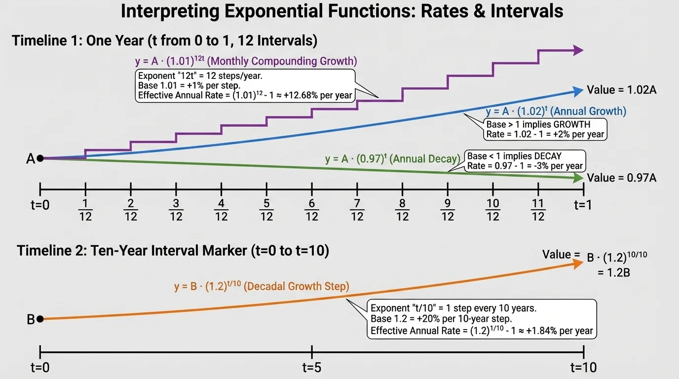
This is why two functions can both show growth but at very different rates. The base alone is not always enough. You must also ask, Over what interval is this multiplier being used?
| Function | Visible factor | Interpretation | Growth or decay |
|---|---|---|---|
| \(y=(1.02)^t\) | \(1.02\) | \(2\%\) increase per time unit | Growth |
| \(y=(0.97)^t\) | \(0.97\) | \(3\%\) decrease per time unit | Decay |
| \(y=(1.01)^{12t}\) | \(1.01\) | \(1\%\) increase repeated \(12\) times per time unit | Growth |
| \(y=(1.2)^{t/10}\) | \(1.2\) | \(20\%\) increase every \(10\) time units | Growth |
Table 1. Interpretations of several exponential functions and their classifications.
Looking back at [Figure 1], you can also connect the algebra to the graph: growth curves rise faster and faster, while decay curves fall quickly at first and then level off toward zero without becoming negative.
A quantity that grows by a small percent very often can outpace a larger-looking percent applied less frequently. That is one reason compound interest can be surprisingly powerful over long periods of time.
That idea appears in science and finance all the time. Frequency matters.
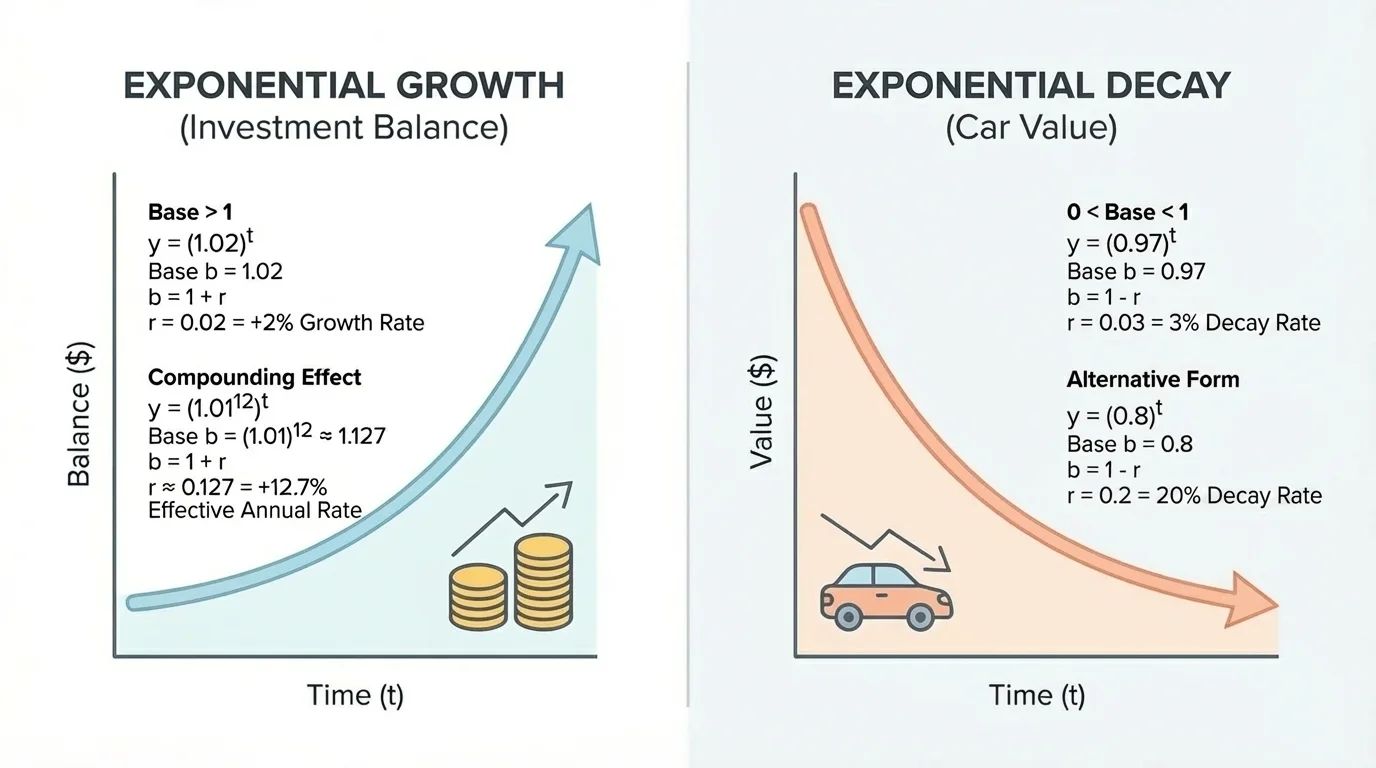
[Figure 4] Exponential models are not just algebra exercises. The same structure can describe money increasing in an account and value shrinking over time in a depreciating object. The interpretation depends on what the variables represent.
If a population grows by \(2\%\) each year, a model like \(P=P_0(1.02)^t\) makes sense. If the value of a machine drops by \(3\%\) each year, a model like \(V=V_0(0.97)^t\) fits instead.
In medicine, a drug in the bloodstream may decay by a fixed percent each hour. In ecology, a species may increase by a fixed percent each season under favorable conditions. In digital technology, repeated percentage growth appears in data storage demand, user adoption, and network expansion.
The function \((1.01)^{12t}\) often appears in finance because interest might be applied monthly while time is measured in years. The function \((1.2)^{t/10}\) can model a quantity that grows by \(20\%\) over each decade if \(t\) is measured in years. Looking again at [Figure 3], the timeline helps explain why these expressions look different even when both represent repeated percent increase.
One common mistake is confusing the initial value with the growth factor. In \(y=5(1.02)^t\), the initial value is \(5\), not \(1.02\). The factor \(1.02\) controls the percent change, while \(5\) tells where the function starts.
Another common mistake is thinking that every base larger than \(1\) gives the percent directly. The percent rate is not \(1.02\%\); it is \(2\%\), found by subtracting \(1\): \(1.02-1=0.02\).
A third mistake is ignoring the exponent structure. In \((1.01)^{12t}\), the growth is not simply \(12\%\) because repeated multiplication is not the same as repeated addition. The true one-unit factor is \((1.01)^{12}\), not \(1+12(0.01)\).
Finally, students sometimes classify \((0.97)^t\) as negative growth because it is decreasing. A better and more precise term is exponential decay. The quantity remains positive, but it gets smaller by a fixed percent each time.
"The form of a function can hide a property or reveal it."
— A central idea in algebra
That is why algebra often asks you to rewrite expressions. You are not just simplifying; you are uncovering meaning.
When you see an exponential expression, ask three questions. What is the initial value? What factor is being applied? Over what time interval is that factor applied? Those questions let you interpret the function whether it is written directly or in a disguised equivalent form.
For a function in the form \(y=a(b)^t\), start with the base. If \(b>1\), think growth. If \(0<b<1\), think decay. Then convert the factor to a percent rate. If the exponent is more complicated than just \(t\), use exponent properties to rewrite the function so the time scale becomes clearer.