A weather app predicts tomorrow's temperature, a navigation app chooses the fastest route, and engineers test bridge designs on computers before building anything. None of these systems relies on guesswork alone. They use representations: equations, graphs, simulations, algorithms, and data models. These representations turn messy reality into something we can analyze, test, and explain.
In science and engineering, a representation is a way of expressing information about a system. Some representations are mathematical, such as an equation like \(d = vt\). Some are computational, such as a spreadsheet or simulation. Some are algorithmic, meaning they give a precise sequence of steps for solving a problem or modeling a process. The power of these tools is that they let us move from observation to explanation. Instead of saying, "It seems to go faster," we can calculate, graph, compare, and justify a claim with evidence.
A mathematical representation expresses a relationship using numbers, variables, equations, graphs, or functions.
A computational representation uses digital tools such as simulations, spreadsheets, or code to model a system or process.
An algorithmic representation describes a process as an ordered set of steps or rules that can be followed consistently.
A model is a simplified representation of a real system used to explain, predict, or design.
These forms of representation overlap. A spreadsheet may contain formulas, a simulation may follow an algorithm, and a graph may summarize the results of a computer model. What matters is not the tool by itself, but how well it helps answer a question or support a claim.
Scientific phenomena often involve change, interaction, and patterns that are hard to see just by looking. A model helps isolate the most important features of a system so that we can reason about it clearly. For example, if we want to explain why a falling object speeds up, we can measure time and velocity, place the data in a table, graph the trend, and write a mathematical relationship between variables.
Representations also help us communicate. A claim such as "the chemical reaction rate increases with temperature" becomes much stronger if it is supported by a graph, a table of measured values, and perhaps a simulation showing particle collisions increasing. In engineering, saying "design A is better than design B" is weak unless the claim is backed by measurable criteria such as cost, strength, efficiency, or safety.
Representations are evidence tools
When scientists and engineers make claims, they are expected to support those claims with evidence and reasoning. Mathematical, computational, and algorithmic representations help organize evidence, reveal relationships, and test whether an explanation matches observed data.
For grades \(9\) to \(12\), an important shift is learning that these representations are not decorations. A graph is not just a picture. An equation is not just a rule to memorize. A simulation is not just animation. Each one is a way to think.
A mathematical representation describes a system using quantities and relationships. As [Figure 1] illustrates, it can show how one variable depends on another, and a graph can reveal patterns of change much faster than a list of numbers can. In many scientific explanations, the goal is to identify variables, determine how they are related, and represent that relationship clearly.
Suppose a cyclist moves at constant speed. If the speed is \(6 \textrm{ m/s}\), then distance after time \(t\) is
\(d = 6t\)
This simple equation tells us several things. Distance and time are proportional. If time doubles, distance doubles. The graph is a straight line through the origin. A table of values also follows the same pattern.
Another example comes from density. If mass is \(m\) and volume is \(V\), then density is
\[\rho = \frac{m}{V}\]
If two objects have the same volume but different masses, the heavier one has a greater density. This allows students to compare substances quantitatively and support explanations about why some materials float and others sink.
Mathematical representations often involve variables. A variable is a symbol, usually like \(x\), \(t\), or \(V\), that stands for a quantity that can change. In science, variables have physical meaning. Time, force, temperature, concentration, and population size can all be variables. Identifying which variable is independent and which is dependent is a basic but crucial skill.
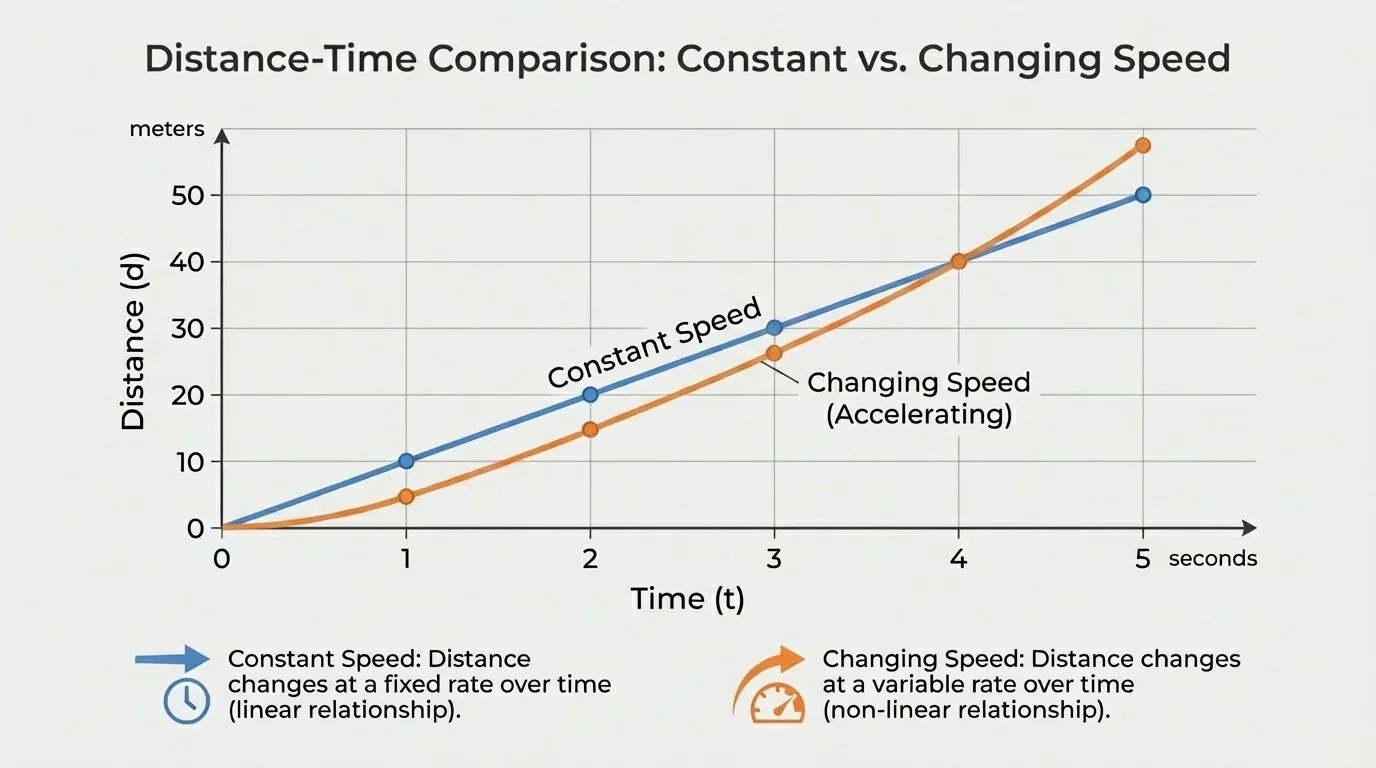
Graphs are especially useful because they make trends visible. A straight line can show constant rate of change. A curved graph can show acceleration, exponential growth, or saturation. The slope of a graph often carries meaning. On a distance-time graph, slope represents speed. On a temperature-time graph, slope represents how quickly temperature changes.
This is why scientists do not rely only on raw data. A table might contain the values \(2\), \(4\), \(6\), \(8\), and \(10\), but without context and relationships, those numbers say little. Once graphed or connected through an equation, the pattern becomes interpretable. Looking back at [Figure 1], the difference between constant and changing motion becomes visually obvious because the shapes of the graphs tell different stories.
From earlier algebra, you already know that equations can represent patterns and that slope measures rate of change. In science, the same ideas apply, but now the symbols represent physical quantities, and the results are used to explain real phenomena.
Many scientific laws are mathematical relationships. Ohm's law is \(V = IR\), where voltage depends on current and resistance. Newton's second law is \(F = ma\), where force depends on mass and acceleration. The ideal gas law, in simplified form, shows that pressure, volume, and temperature are connected. Students are not just expected to calculate with these equations, but to explain what the equations mean.
A computational representation uses a computer to carry out many calculations quickly, organize large sets of data, or simulate systems that are difficult to solve by hand. Many computational models work by starting with initial values, applying rules, updating the system, and repeating the process many times.
Why is this useful? Some systems are too complex for a single neat equation. Weather depends on temperature, pressure, moisture, wind, landforms, and time. Disease spread depends on contact patterns, immunity, incubation, and behavior. Traffic flow depends on speed, spacing, lane changes, and signals. A computer can apply the same rules repeatedly to many interacting parts.
This repeated process is called iteration. In an iterative model, one cycle produces updated values, and those values become the starting point for the next cycle. For example, if a population grows by \(5\%\) each year, and starts at \(1{,}000\), then after one year it is \(1{,}000 \times 1.05 = 1{,}050\). After two years it is \(1{,}050 \times 1.05 = 1{,}102.5\). A computer can continue this process for hundreds of steps almost instantly.
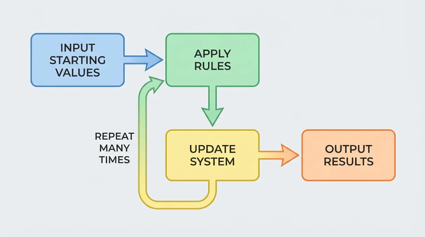
[Figure 2] Spreadsheets are one of the simplest computational tools available to students. A spreadsheet can calculate ratios, generate graphs, fit trend lines, and test "what-if" questions. If a student changes one variable, the whole table updates. This makes it easier to investigate how systems respond to changes.
Computer simulations are even more powerful. A simulation might model particles moving in a gas, predators and prey in an ecosystem, or energy use in a building. Although simulations can look impressive, they still rely on assumptions and rules chosen by humans. Their results are only as reliable as the model behind them. That is why computational outputs must be interpreted, not merely accepted.
Later, when discussing uncertainty, it helps to remember [Figure 2]: each loop in a simulation depends on both previous outputs and the rules built into the model. If the starting values or rules are unrealistic, repeated iteration can produce misleading predictions.
An algorithmic representation expresses a process as clear, ordered steps. Algorithms are common in computer science, but they also appear throughout science and engineering. A lab procedure is algorithmic. A troubleshooting checklist is algorithmic. A method for solving a quadratic equation is algorithmic.
An algorithm must be precise enough that someone else, or a computer, could follow it and get the same kind of result. Consider a simple algorithm for determining average speed:
Step sequence: measure distance, measure time, divide distance by time, report the result with units. Mathematically, this is \(v = \dfrac{d}{t}\), but the algorithm tells how to obtain and use the values.
Algorithms often include decisions. For example: if the measured value is outside an expected range, repeat the trial; otherwise, record it. In coding, such a rule is a conditional statement. In engineering, it may become a design test. In daily life, a navigation app follows an algorithm that compares routes, estimates travel times, and updates when traffic changes.
Search engines, music recommendations, and social media feeds all rely on algorithms. The same core idea of step-by-step rule following is also used in science to sort data, model systems, and control machines.
Algorithmic thinking is valuable because it forces precision. If an explanation is too vague to turn into steps, it may also be too vague to test. When students create a process for analyzing data or comparing designs, they are turning reasoning into a form that others can examine and repeat.
One of the most important scientific skills is using representations to connect data to a claim. Data by themselves are observations or measurements. A claim is an answer to a question. The representation provides the bridge.
Suppose students investigate whether light intensity affects plant growth. They measure the height of plants under three light levels over three weeks. The raw measurements go into a table. Then averages are calculated. Then a graph is made. If the graph shows that higher light intensity is associated with greater average growth, the claim is supported. The graph does not prove everything, but it gives structured evidence.
| Light level | Average growth after \(3\) weeks |
|---|---|
| Low | \(4.2 \textrm{ cm}\) |
| Medium | \(7.1 \textrm{ cm}\) |
| High | \(9.4 \textrm{ cm}\) |
Table 1. Average plant growth under three different light levels.
From this table, a student can argue that growth increases as light level increases. A stronger explanation might add biological reasoning, such as the role of light in photosynthesis, but the representation makes the trend visible and measurable.
Sometimes the evidence is not perfectly neat. Real data often contain scatter. This is why trend lines, averages, and repeated trials matter. A single unusual measurement does not automatically destroy a claim, but it should lead students to ask whether there was error, variation, or another factor involved.
Claims need both pattern and reasoning
A graph or equation supports a claim by showing a pattern, but students must still explain why the pattern makes sense. Strong explanations combine the representation with scientific principles, not just a description of what the graph looks like.
For example, a graph showing that reaction rate increases with temperature supports the claim that heating speeds reactions. The explanation becomes stronger when students connect the pattern to particle motion and collision frequency. In other words, the representation supports the claim, and scientific reasoning explains the cause.
[Figure 3] Representations are not only for explaining natural phenomena. They are also essential for engineering design. Engineers often compare several possible solutions under constraints such as cost, mass, efficiency, durability, or environmental impact. A strong design decision usually depends on comparing multiple variables at once rather than focusing on only one.
Suppose a team is designing a bicycle frame. Aluminum may be light and affordable, steel may be strong and cheap but heavier, and carbon fiber may be very light and strong but expensive. A table or chart can help compare materials quantitatively. This makes the design process more objective.
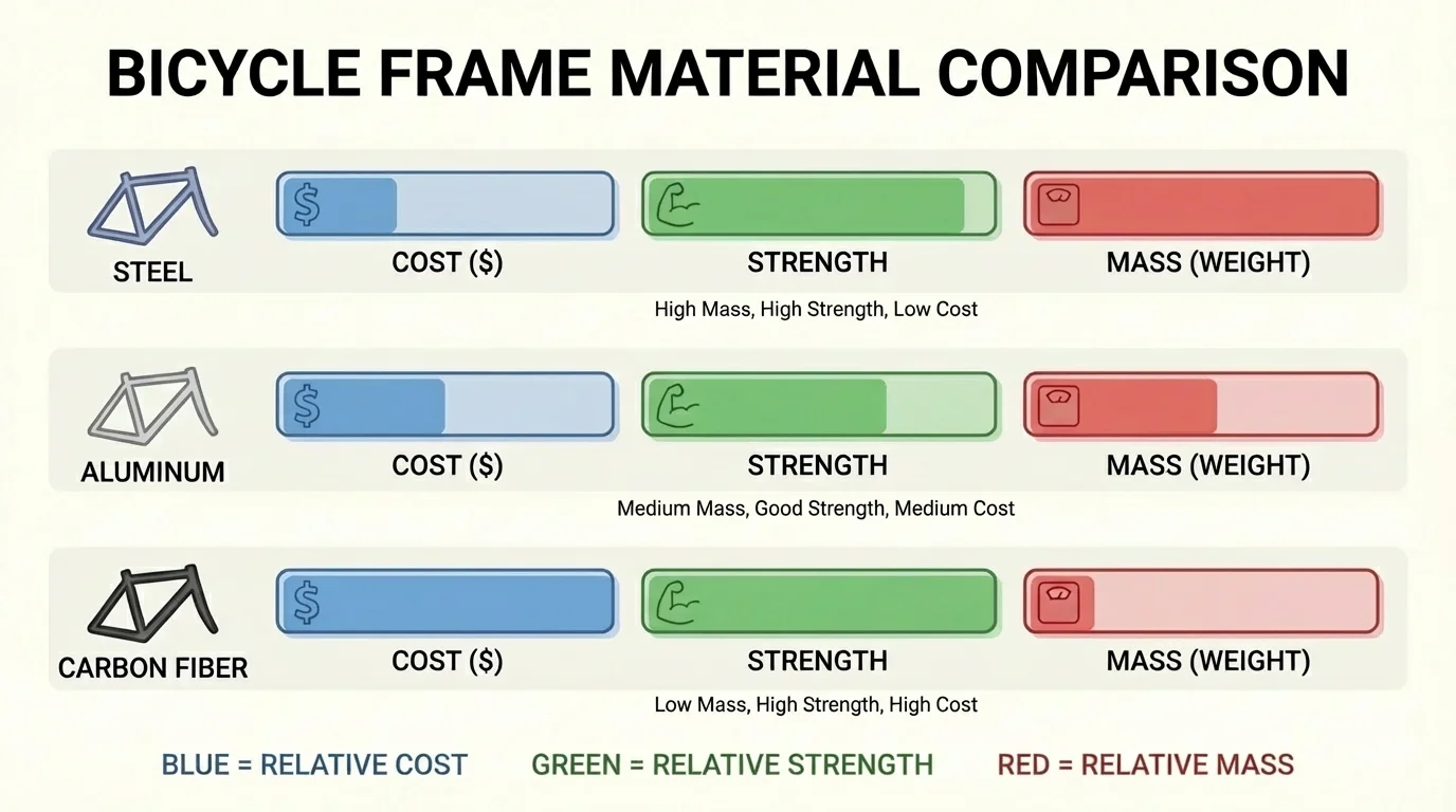
Optimization means finding the best solution according to chosen criteria. In some cases, "best" means minimum cost. In others, it means maximum efficiency or the best balance among trade-offs. A solution that is strongest may also be heaviest. A solution that is cheapest may wear out quickly. Quantitative representations let students justify why one option is better for a specific purpose.
Decision matrices are useful here. A design team can assign weights to criteria and calculate scores. For example, if safety is twice as important as cost, the scoring system should reflect that. This turns vague preferences into a structured argument.
When students refer back to [Figure 3], they can see why engineering is rarely about one perfect answer. It is about evidence-based choices under constraints. The chart format helps reveal trade-offs that would be easy to miss in a long paragraph.
No representation captures every detail of reality. Every model simplifies. That is a strength, because simplification makes reasoning possible, but it is also a limitation. A mathematical formula may ignore friction. A simulation may assume uniform temperature. An algorithm may classify based on incomplete data.
An assumption is something treated as true in order to build or use a model. Assumptions should be stated clearly. For example, the equation \(d = vt\) assumes constant speed. If speed changes, the equation no longer fully describes the motion. Likewise, a population model may assume constant growth rate, even though real populations are affected by food, disease, and migration.
Uncertainty is also unavoidable in measurement and modeling. Measurements can vary because of instrument limits, human error, or natural variation. Computational models may produce different results if starting conditions change slightly. Understanding uncertainty does not weaken science; it makes explanations more honest and more precise.
"All models are wrong, but some are useful."
— George Box
This famous statement captures an important truth. A model is not judged by whether it copies reality perfectly. It is judged by whether it helps explain, predict, or design effectively for a specific purpose.
In climate science, mathematical and computational representations are used to estimate how atmospheric gases affect global temperature. Scientists track variables such as carbon dioxide concentration, ocean temperature, and ice cover. They use equations and simulations together because the climate system is too complex for a single simple formula.
In epidemiology, disease spread can be represented with rates of transmission and recovery. A basic model might track how many people are susceptible, infected, or recovered over time. Small changes in the transmission rate can lead to very different outcomes, which is why computational models are so important for public health planning.
In transportation, route-planning systems use algorithms to compare travel times, update predictions, and redirect vehicles. In energy engineering, designers use models to calculate efficiency, heat loss, and power consumption. In sports science, data from motion sensors can be represented in graphs to improve running technique or analyze how quickly an athlete accelerates.
Modern aircraft are tested in computer simulations long before full-scale prototypes fly. Engineers save time, reduce cost, and improve safety by using models to detect weak points early.
These examples all share the same core idea: representations help humans reason about systems that are too fast, too large, too small, too complex, or too expensive to understand by observation alone.
The best way to see the value of these tools is to watch how they support a claim or design decision step by step.
Worked example 1: Using an equation to support a motion claim
A student claims that a cart moving at constant speed travels \(18 \textrm{ m}\) in \(3 \textrm{ s}\), so its speed is \(6 \textrm{ m/s}\).
Step 1: Choose the relationship
For constant speed, use \(v = \dfrac{d}{t}\).
Step 2: Substitute the values
\(v = \dfrac{18}{3} = 6\).
Step 3: Interpret the result
The speed is \(6 \textrm{ m/s}\), which means the cart travels \(6 \textrm{ m}\) each second.
The claim is supported because the measured distance and time match the calculated speed: \[v = 6 \textrm{ m/s}\]
This example is simple, but it shows a key point: a numerical claim becomes stronger when it is tied to a clear mathematical relationship.
Worked example 2: Interpreting a rate from data
A tank contains \(120 \textrm{ L}\) of water and loses \(15 \textrm{ L}\) every minute. Represent the amount of water after \(t\) minutes and predict the amount after \(4\) minutes.
Step 1: Write the relationship
The amount decreases linearly, so \(W = 120 - 15t\).
Step 2: Substitute \(t = 4\)
\(W = 120 - 15(4) = 120 - 60 = 60\).
Step 3: Interpret the slope
The value \(-15\) is the rate of change, meaning the tank loses \(15 \textrm{ L}\) each minute.
After \(4\) minutes, the tank contains: \[W = 60 \textrm{ L}\]
Notice that this equation does more than compute one answer. It describes the whole process and can be graphed to show a straight decreasing line.
Worked example 3: Simple computational iteration
A bacteria culture starts with \(500\) cells and grows by \(20\%\) each hour. Use iterative reasoning to find the population after \(3\) hours.
Step 1: Apply the growth factor once
After \(1\) hour: \(500 \times 1.2 = 600\).
Step 2: Repeat the same rule
After \(2\) hours: \(600 \times 1.2 = 720\).
Step 3: Repeat again
After \(3\) hours: \(720 \times 1.2 = 864\).
The iterative model predicts a population of \(864\).
This is a computational way of thinking because the same rule is applied again and again. A spreadsheet or short program would do the same thing for many more time steps.
Worked example 4: Comparing design choices quantitatively
A phone case is being designed with two materials. Material A costs $8, has a protection score of \(7\), and mass \(40 \textrm{ g}\). Material B costs $12, has a protection score of \(9\), and mass \(35 \textrm{ g}\). If protection matters most, which material is easier to justify?
Step 1: Identify the key criteria
The design considers cost, protection, and mass.
Step 2: Compare the values
Material B has higher protection: \(9 > 7\). It is also lighter: \(35 < 40\), but more expensive.
Step 3: Link the evidence to the goal
If protection is the top priority, the gain from \(7\) to \(9\) may justify paying $4 more.
A reasonable claim is that Material B is the better design choice when safety and protection are weighted more heavily than cost.
Examples like these show that representations are not only for calculation. They are tools for explanation, prediction, comparison, and decision-making.
Different questions call for different tools. A table is useful for recording measurements. A graph is useful for spotting trends. An equation is useful for expressing a precise relationship. A simulation is useful for systems with many interacting parts. An algorithm is useful when the process itself needs to be clear, repeatable, and testable.
Good scientists and engineers often move between representations. They may start with data in a table, graph the data, infer a relationship, write an equation, and then use a computer model to test what happens under new conditions. Each form adds something different.
The most convincing explanations and design arguments do not depend on a single representation. They combine them. A claim supported by data, graph, equation, and reasoning is much stronger than a claim supported only by opinion.