Two classes can do the same science activity and still get slightly different results. One class might find that bean plants in sunlight grow to about \(18\) centimeters, while another class measures \(17\) centimeters. Does that mean one class is wrong? Not always. Learning how to analyze and interpret data helps us figure out what the results really mean. It helps us notice what is the same, what is different, and why those patterns might happen.
People use data all the time, even outside science. Coaches compare scores from different games. Meteorologists compare temperatures from different days. Doctors compare heart rate readings. Students compare survey answers. In each case, people are not just collecting numbers. They are studying those numbers to find patterns and make smart decisions.
Data are pieces of information that we collect. Data can be numbers, words, measurements, counts, or observations. For example, if students count how many birds land near the playground, those counts are data. If they describe the birds as small, gray, or noisy, those descriptions are also data.
A finding is what we learn from data after studying it. If a class records the heights of plants and notices that plants near sunlight are taller, that is a finding. Data are the information we gather. Findings are the ideas we discover from that information.
Data are collected facts, numbers, measurements, or observations.
Findings are the results or ideas we learn after studying data.
Analyze means to examine data carefully.
Interpret means to explain what the data show.
Sometimes data are called observations when they come from noticing with our senses, and sometimes they are called measurements when they are found with tools such as rulers, scales, or thermometers. A count of \(12\) ladybugs is data. A water temperature of \(22\) degrees Celsius is also data.
Raw data can look messy at first. A page full of numbers is hard to understand. Organized displays make patterns easier to see, as [Figure 1] shows with plant data arranged in a table and graph. When data are grouped clearly, we can compare one set of findings with another much more easily.
Good data organization includes labels, units, and clear categories. If plant height is measured in centimeters, the table should say so. If students compare plants in sunlight and shade, the categories should be named clearly. Without labels, a number such as \(15\) does not tell us enough. Is it \(15\) centimeters, \(15\) grams, or \(15\) days?
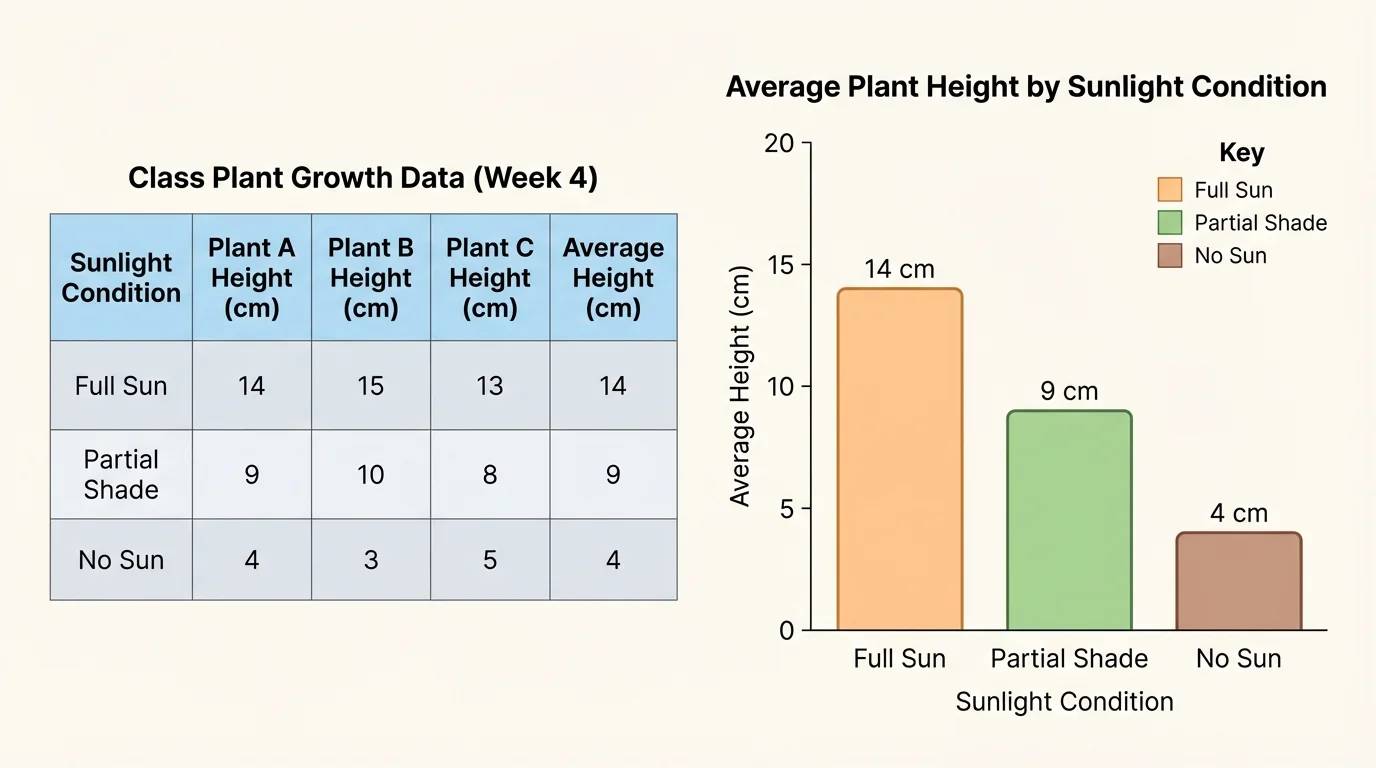
A table is useful when you want to read exact values. A graph is useful when you want to notice patterns quickly. For example, look at this sample data about plant height after one week.
| Group | Plant A | Plant B | Plant C | Average Height |
|---|---|---|---|---|
| Sunlight | \(18\) | \(17\) | \(19\) | \(18\) |
| Shade | \(11\) | \(12\) | \(10\) | \(11\) |
Table 1. Plant heights in centimeters for plants grown in sunlight and shade.
From this table, we can already notice a similarity and a difference. The plants within each group are close in height, which is a similarity inside each group. But the sunlight group is taller than the shade group, which is a difference between the groups.
To compare data fairly, remember to check that the same kind of measurement is being used. Comparing \(12\) centimeters with \(12\) inches is not fair unless the units are changed to match.
Neat organization also helps us spot mistakes. If one plant height were written as \(180\) centimeters after just one week, that would look unusual. The organized table helps us question whether it was measured incorrectly or written down wrong.
When we look for similarities, we ask: What parts of the data match or nearly match? Do two groups show the same pattern? Are the values close together? Do the results repeat in more than one trial?
Suppose students test which surface lets a toy car roll farthest. They run the car on tile, carpet, and wood three times each. If the car rolls far on tile every time, that repeated pattern is a similarity across the trials. Repeated patterns make findings stronger because they happen more than once.
Similarities can appear in different ways. Two groups may both increase over time. Two graphs may both have the tallest bar in the same category. Two experiments may both show that more sunlight helps plants grow better. We should not only look for exact matches. Results that are close can still show a useful similarity.
Patterns matter more than single numbers. One number by itself does not tell the whole story. When several data points point in the same direction, we begin to see a pattern. Scientists trust patterns more than one isolated result.
For example, imagine two classes measuring the number of worms found in moist soil and dry soil. If one class finds \(14\) worms in moist soil and \(5\) in dry soil, and the other class finds \(16\) in moist soil and \(6\) in dry soil, the exact counts are not identical. But the pattern is similar: both classes found more worms in moist soil.
Differences are also important. We ask: Which group has more? Which has less? How much more or less? Is one result much higher than the others? Is there an outlier, which is a value that is far away from most of the other values?
If students survey favorite fruits and find that \(20\) students choose apples while only \(7\) choose pears, the difference is easy to notice. But it helps to say the difference clearly. We can calculate it by subtracting: \(20 - 7 = 13\). Apples were chosen by \(13\) more students than pears.
Sometimes differences are small. If one group measures a paper airplane flying \(4.8\) meters and another measures \(5.1\) meters, the difference is \(5.1 - 4.8 = 0.3\) meters. That is a difference, but it is not a very large one. When interpreting data, it helps to notice whether a difference is big enough to matter.
We also compare highest and lowest values. In a week of weather data, the highest temperature might be \(29\) degrees and the lowest might be \(21\) degrees. The range is the difference between the highest and lowest values: \(29 - 21 = 8\). Range tells us how spread out the data are.
Words such as more, less, about the same, and much greater are useful, but numbers make comparisons stronger. We can compare data using totals, differences, and averages.
A average gives a typical value for a set of numbers. One common average is the mean. To find it, add the values and divide by how many values there are.
Worked example 1: Comparing with a difference
A class counts birds at two times of day. In the morning they see \(18\) birds. In the afternoon they see \(11\) birds. How many more birds are seen in the morning?
Step 1: Identify the larger and smaller numbers.
The larger number is \(18\). The smaller number is \(11\).
Step 2: Subtract to find the difference.
\(18 - 11 = 7\)
The finding is that the class sees \(7\) more birds in the morning than in the afternoon.
Now look at an average. Suppose a plant is measured on three days and its heights are \(12\), \(14\), and \(16\) centimeters. The mean is found by adding and dividing:
Worked example 2: Finding an average
Find the mean of \(12\), \(14\), and \(16\).
Step 1: Add the values.
\(12 + 14 + 16 = 42\)
Step 2: Divide by the number of values.
There are \(3\) values, so \(42 \div 3 = 14\).
The average height is \(14\) centimeters.
Averages are helpful because one group may have many data points. Instead of comparing every number one by one, we can compare average values. Earlier, the sunlight plants had an average height of \(18\) centimeters, while the shade plants had an average of \(11\) centimeters. The average difference is \(18 - 11 = 7\) centimeters. That supports the finding that sunlight plants grew taller. As we saw in [Figure 1], graphs make that difference easy to notice quickly.
Worked example 3: Comparing two averages
Group A throws a ball distances of \(6\), \(8\), and \(7\) meters. Group B throws \(4\), \(5\), and \(6\) meters. Which group throws farther on average?
Step 1: Find Group A's mean.
\(6 + 8 + 7 = 21\), and \(21 \div 3 = 7\).
Step 2: Find Group B's mean.
\(4 + 5 + 6 = 15\), and \(15 \div 3 = 5\).
Step 3: Compare the means.
\(7 - 5 = 2\)
Group A throws farther on average by \(2\) meters.
Sometimes it is also useful to compare parts of a whole. If \(8\) out of \(10\) seeds sprout, the fraction is \(\dfrac{8}{10}\), which can also be written as \(\dfrac{4}{5}\). If another group gets \(5\) out of \(10\), or \(\dfrac{5}{10}\), then the first group has a greater sprouting rate.
[Figure 2] Graphs help us see patterns fast. A bar graph can compare categories, and a line graph can show change over time. The labels on the axes and the sizes of the bars or line movements reveal similarities and differences.
When reading a graph, first check the title. Then check the labels on the horizontal and vertical axes. Finally, compare the heights of the bars or the points on the line. If the graph is not labeled clearly, it is easy to misunderstand the data.
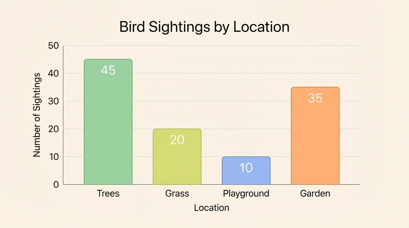
Suppose a bar graph shows bird sightings in four schoolyard habitats: trees \(= 15\), grass \(= 9\), playground \(= 4\), and garden \(= 13\). We can interpret this graph in several ways. Trees and garden have similar counts because \(15\) and \(13\) are close. Playground is very different from the others because \(4\) is much lower.
Line graphs help when we want to see increase, decrease, or no change. If a line graph shows daily temperature for five days as \(20\), \(22\), \(24\), \(23\), and \(25\), then we can say the temperature generally rises, even though it dips a little from \(24\) to \(23\).
A table may be better than a graph when exact values matter most. A graph may be better when the overall pattern matters most. Strong data readers know how to use both. Later, when comparing two investigations, we can return to [Figure 2] and notice that the shape of the data matters, not just one category by itself.
[Figure 3] Sometimes two investigations seem to study the same thing but end with different results. That can happen for good reasons. Interpreting data means thinking about what may have caused the difference, not just noticing that a difference exists.
One reason is variables. A variable is something that can change in an investigation. If one group gives a plant more water, uses different soil, or places it in a warmer room, those variables may affect the findings. For a fair test, scientists try to change only one important variable at a time.
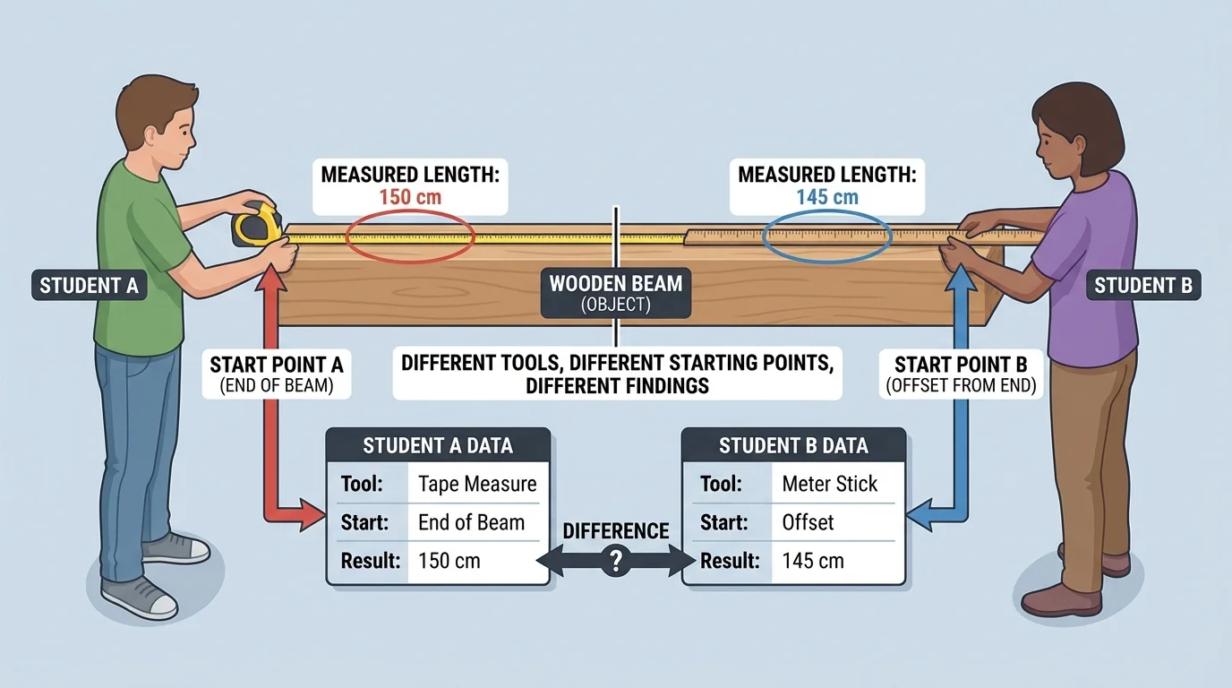
Another reason is measurement error. One student may start measuring from the edge of a ruler instead of the zero mark. One thermometer may be read too quickly. Small mistakes can create slightly different data.
The number of trials also matters. If you toss a coin only \(2\) times, you might get unusual results. If you toss it \(20\) times, the results are usually more dependable. More data often make findings stronger because patterns become clearer.
A result can be different without being wrong. In real science, repeated investigations often produce values that are close but not exactly the same, and scientists study those differences carefully.
Sample size matters too. If only \(3\) students answer a survey, the results may not represent the whole grade. If \(60\) students answer, the data are usually more useful. When interpreting findings, ask whether enough data were collected to support the conclusion.
These ideas help explain why one class may record a plant average of \(18\) centimeters and another class may record \(17\) centimeters. The overall pattern may still match. Just as [Figure 3] highlights method differences, different tools, timing, or small errors can lead to slightly different findings while still supporting the same big idea.
When comparing two investigations, begin by checking whether they measured the same thing in the same way. Did both groups use the same units? Did both collect data for the same amount of time? Were the categories the same?
For example, suppose two classes study how many minutes students read each night. Class A reports \(10\), \(15\), \(20\), \(25\), and \(30\) minutes. Class B reports \(12\), \(18\), \(19\), \(26\), and \(29\) minutes. The findings are similar because both classes have values in about the same range, and both show that many students read around \(20\) to \(30\) minutes.
Now suppose another class reports reading time in hours instead of minutes. Then we must convert the units before comparing. For example, \(1\) hour equals \(60\) minutes. Without matching units, our comparison may be unfair or confusing.
It is also important to compare shape and spread, not only single numbers. Two groups can have the same average but very different data. One group might have \(5\), \(5\), and \(5\). Another group might have \(1\), \(5\), and \(9\). Both have an average of \(5\), but the second group is much more spread out.
A good conclusion is based on evidence from data, not on guessing. It uses words such as the data show, the results suggest, or most of the evidence supports. These phrases remind us to stay close to what the data actually say.
For example, a weak conclusion would be: Sunlight is always perfect for every plant. That statement is too broad. A stronger conclusion would be: In this investigation, plants in sunlight grew taller than plants in shade by an average of \(7\) centimeters. That conclusion uses specific evidence.
"Good conclusions are built from evidence, not guesses."
Sometimes a careful conclusion must include uncertainty. If the results are mixed, we should say so. For example: The data do not show a clear winner because the two groups had very similar averages. Honest interpretation is more important than trying to force a dramatic answer.
When possible, mention both similarities and differences. For example: Both classes found more worms in moist soil than in dry soil, but Class B counted \(2\) more worms overall than Class A. This kind of sentence shows deeper thinking because it compares more than one feature of the findings.
Analyzing data is not only for science labs. Weather experts compare rainfall from different months. Stores compare how many items sell in summer and winter. Doctors compare a patient's temperature over several days. Wildlife scientists compare animal counts in different habitats. In each case, people look for patterns, similarities, and differences before making decisions.
Sports provide another clear example. A basketball coach may compare free-throw results from two weeks of practice. If one week the team makes \(42\) out of \(60\) shots and the next week makes \(51\) out of \(60\), the coach can see improvement. The difference is \(51 - 42 = 9\) more successful shots, and the fraction of made shots increased from \(\dfrac{42}{60}\) to \(\dfrac{51}{60}\).
At school, student councils may use surveys to find favorite lunch choices or preferred spirit-day themes. If two survey groups give similar answers, leaders can feel more confident about the result. If answers differ a lot, they may need more data before deciding.
One common mistake is noticing only one number and ignoring the rest of the data. A single high score or low score may not represent the full pattern. Another mistake is forgetting units. A length in centimeters and a length in meters are not directly comparable until the units match.
A third mistake is confusing correlation with proof. If two things happen together, that does not always mean one caused the other. For example, if more students bring jackets on rainy days, the jackets did not cause the rain. The rain likely caused the jackets.
Another mistake is using words such as always or never when the data do not support such strong claims. Data often suggest patterns, but careful thinkers know that evidence has limits.
Finally, do not ignore unusual values. If one result is very different, ask why. It may be an error, or it may point to something important. Good analysis includes questioning surprising data instead of hiding them.