A weather app predicts rain, a doctor studies disease spread, and an engineer tests whether a bridge design is safe. None of these people can directly see the future, yet they still make decisions that matter. How? They use data and models. In science, this combination is powerful: carefully analyzed data reveal patterns, and computational models help scientists test explanations, estimate what might happen next, and decide whether a claim is strong enough to trust.
Modern science rarely depends on a single measurement or one graph. Instead, scientists work with datasets, compare variables, check uncertainty, and build models that simulate how a system behaves. A model does not magically produce truth. It is only as good as the evidence, assumptions, and methods behind it. That is why learning to analyze data with computational models is really about learning to think scientifically.
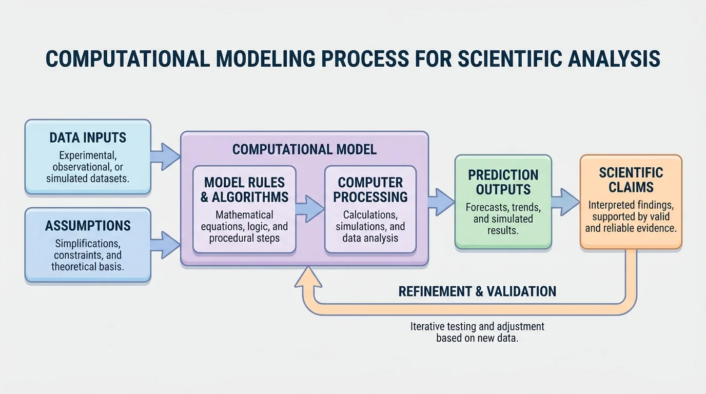
[Figure 1] Science often deals with systems too large, too small, too fast, too slow, or too complex to study by direct observation alone. Climate systems involve oceans, atmosphere, ice, and solar energy. Population changes involve birth rates, food supply, competition, and disease. Chemical reactions may happen at rates that depend on temperature and concentration. In each case, raw observations are important, but they are not enough. Scientists need a way to organize evidence and test how variables interact.
A computational model is a model that uses calculations, rules, or algorithms, usually on a computer, to represent a real system. It takes inputs, applies assumptions and mathematical relationships, and produces outputs such as predictions, simulations, or trend estimates. For example, a model of bacterial growth might begin with an initial population, apply a growth rule each hour, and estimate the number of bacteria after one day.
Computational models are useful because they let scientists test many scenarios quickly. They can ask, "What happens if the temperature rises by \(2^\circ \textrm{C}\)?" or "What if the infection rate drops by half?" A good model helps scientists compare possibilities, but it never replaces real data. Instead, the strongest science comes from using models and observations together.
Scientific data analysis means more than reading numbers off a table. It includes organizing data, displaying them in graphs, calculating useful quantities, looking for trends, comparing groups, identifying unusual points, and deciding whether patterns are meaningful. Scientists ask questions such as: Is one variable increasing as another decreases? Does the pattern look linear, exponential, cyclic, or random? Are there outliers? Are repeated measurements consistent?
Suppose students measure the cooling of hot water every \(2\) minutes. The data might be placed in a table and plotted on a graph of temperature versus time. If the temperature drops quickly at first and then more slowly, the graph suggests that the cooling rate changes over time. That pattern can guide the choice of model.
Scientists also distinguish between independent variables and dependent variables. The independent variable is the one that is changed or used for comparison, while the dependent variable is what is measured in response. In a plant growth experiment, time or fertilizer amount might be the independent variable, and plant height might be the dependent variable.
When reading a graph, always check the axes, units, and scale first. A graph can look dramatic or unimportant simply because of how the axes are chosen.
Another important part of analysis is identifying outliers, data points that differ strongly from the overall pattern. An outlier could signal a measurement mistake, a special event, or a real but rare effect. Scientists do not automatically delete outliers. They investigate them.
Not all models are the same. A physical model is a tangible representation, like a globe. A conceptual model explains relationships in words or diagrams. A computational model uses calculations and rules to simulate behavior over time or under changing conditions. In many scientific fields, computational models are especially important because they can handle large datasets and repeated calculations.
Most computational models have four basic parts. First, they use inputs, which are starting values or measured data. Second, they include assumptions, which simplify reality. Third, they apply rules or equations that describe how the system changes. Fourth, they produce outputs, such as tables, graphs, or predicted values. If a lake pollution model assumes perfect mixing of water, that assumption may make the model easier to compute, but less realistic in some situations.
Scientists choose models based on the kind of pattern they expect. A straight-line trend may suggest a linear model. Rapid growth may suggest an exponential model. A repeated rise-and-fall pattern may suggest a cyclic model. Sometimes the correct model is not obvious at first, so scientists test multiple models and compare which one fits the data better.
A valid claim is a scientific statement that is well supported by appropriate evidence and sound reasoning. A reliable claim is based on data and methods that produce consistent results when repeated or checked independently.
The difference matters. A result could be reliable but not valid if the same mistake happens every time. For example, if a temperature probe is incorrectly calibrated and always reads \(2^\circ \textrm{C}\) too high, repeated trials may be consistent, but the conclusion based on those values is still wrong.
Science is not just collecting numbers; it is building explanations. A scientific claim should connect three parts: the claim itself, the evidence, and the reasoning. The claim is the statement being made. The evidence is the analyzed data. The reasoning explains why the evidence supports the claim and how the model connects the two.
For example, consider a claim that a certain fertilizer increases plant growth. The evidence might be that treated plants reached an average height of \(18 \, \textrm{cm}\) while untreated plants reached \(12 \, \textrm{cm}\) after the same number of days. The reasoning must then explain why the difference matters, whether the sample size was adequate, whether other conditions were controlled, and whether a model of growth supports the conclusion.
A weak claim often goes beyond the data. If a model predicts a trend for \(10\) days, claiming it proves what will happen for a year is risky unless the model has been validated over longer times. Strong claims stay close to the evidence and clearly state limitations.
Claims must match the scope of the model
A model can only support claims within the conditions and assumptions built into it. If a disease-spread model assumes a closed school with no new students entering, then its predictions do not automatically apply to an open city-wide population. Scientists make stronger arguments when they say exactly what the model can and cannot support.
This is one reason scientific language often sounds careful. Words such as suggests, supports, is consistent with, and under these conditions are not signs of weakness. They are signs of precision.
Validity asks whether a method or claim actually measures or explains what it is supposed to measure or explain. Reliability asks whether the results are consistent across repeated trials or repeated analyses. Good science aims for both.
Several factors affect validity. These include biased sampling, poor control of variables, incorrect assumptions, faulty instruments, and using a model outside the situation it was designed for. Reliability can be reduced by random measurement error, inconsistent procedures, or too little data.
Scientists also think about uncertainty. Every measurement has some uncertainty because no instrument is perfectly exact. If a ruler measures to the nearest millimeter, then lengths recorded from that ruler carry a limited precision. If a temperature sensor varies by \(\pm 0.5^\circ \textrm{C}\), then the data should be interpreted with that uncertainty in mind.
Suppose a sensor gives temperature readings of \(24.1^\circ \textrm{C}\), \(24.3^\circ \textrm{C}\), and \(24.2^\circ \textrm{C}\). The average is \(\dfrac{24.1 + 24.3 + 24.2}{3} = 24.2^\circ \textrm{C}\). These values are close together, so the measurements appear reliable. But if the sensor is poorly calibrated and the true temperature is \(23.0^\circ \textrm{C}\), the measurements are not valid.
Some famous scientific errors were caused not by weak mathematics but by hidden assumptions. A model can produce neat graphs and still be misleading if the assumptions do not match the real world.
Because of this, scientists test instruments, repeat trials, compare independent data sources, and revise models when the evidence demands it.
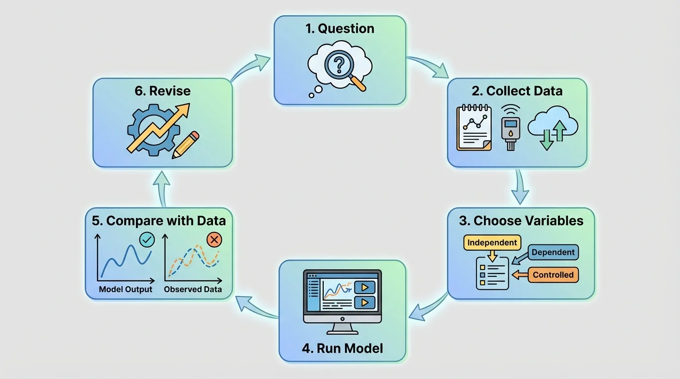
[Figure 2] The modeling process follows a cycle: define a question, choose variables, gather data, build rules, run the model, compare outputs with real observations, and revise if needed. This cycle is one of the clearest examples of analyzing and interpreting data in science because each stage depends on evidence.
First, scientists identify the question. For instance: How fast does a population of insects grow in a container? Next, they select variables such as starting population, food amount, and time. Then they choose a rule. A simple first model might assume the population doubles every day. That rule may be unrealistic, but it gives a starting point.
After running the model, scientists compare predictions to actual data. This comparison is called validation. If the model predicts \(160\) insects after four days but the observed count is only \(92\), the model may need revision. Perhaps food becomes limited, so the growth rate slows.
Sometimes scientists also calibrate a model. Calibration means adjusting model parameters so that the model better matches observed data. For example, instead of assuming a daily growth factor of \(2.0\), a scientist might test values like \(1.3\), \(1.4\), or \(1.5\) and see which one fits best.
A strong model is not one that looks complicated. It is one that captures the key behavior of the system, matches evidence reasonably well, and makes testable predictions.
[Figure 3] Suppose a scientist studies insects in a controlled container. The observed population counts over five days are \(20\), \(28\), \(39\), \(55\), and \(77\). A simple growth model predicts that each day the population is multiplied by \(1.4\). Comparing the predicted values to the observed values helps test whether the model is useful.
Case study: testing a simple growth rule
Step 1: Start with the initial value
Let the initial population be \(P_0 = 20\).
Step 2: Apply the model repeatedly
Use \(P_{n+1} = 1.4P_n\).
Day \(1\): \(P_1 = 1.4 \times 20 = 28\)
Day \(2\): \(P_2 = 1.4 \times 28 = 39.2\)
Day \(3\): \(P_3 = 1.4 \times 39.2 = 54.88\)
Day \(4\): \(P_4 = 1.4 \times 54.88 = 76.832\)
Step 3: Compare the model with observed data
The predictions \(28\), \(39.2\), \(54.88\), and \(76.832\) are very close to the observations \(28\), \(39\), \(55\), and \(77\).
This supports the claim that, under these conditions, a growth factor near \(1.4\) per day is a reasonable model.
The key idea is not that the model is perfect. Real populations do not keep growing at the same rate forever. But for this short time interval, the model fits well enough to support a limited, valid claim.
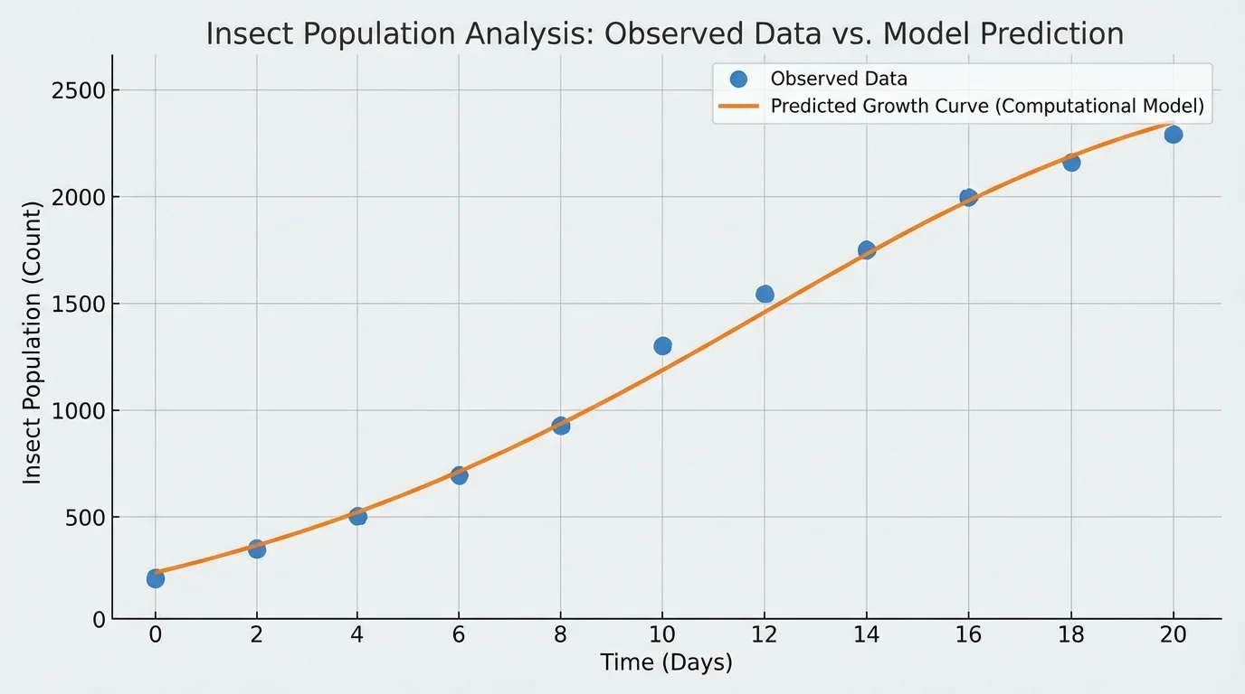
Later, if food runs low, the same model may fail. That does not mean modeling is useless. It means claims must match the time range and assumptions of the model. The population comparison in the graph makes this especially clear: good agreement over a few days does not guarantee good agreement forever.
Now consider a cup of hot tea cooling in a room. The rate of cooling depends on the difference between the tea temperature and room temperature. A simple computational rule might say that every minute, the temperature moves \(20\%\) of the way from its current value toward room temperature.
Case study: a simple cooling model
Step 1: Set the starting values
Suppose the tea starts at \(80^\circ \textrm{C}\) and the room is \(20^\circ \textrm{C}\).
Step 2: Apply the rule for one minute
The difference from room temperature is \(80 - 20 = 60^\circ \textrm{C}\).
Twenty percent of that is \(0.2 \times 60 = 12^\circ \textrm{C}\).
So the new temperature is \(80 - 12 = 68^\circ \textrm{C}\).
Step 3: Apply the rule again
The new difference is \(68 - 20 = 48^\circ \textrm{C}\).
Twenty percent of that is \(0.2 \times 48 = 9.6^\circ \textrm{C}\).
The next temperature is \(68 - 9.6 = 58.4^\circ \textrm{C}\).
The model predicts rapid cooling at first and slower cooling later, which matches what people often observe in everyday life.
If observed temperatures are close to these predictions, the model supports the claim that this simple cooling rule is useful for the situation. If the cup is stirred, covered, or placed in a refrigerator, the model may need new assumptions and new parameters.
A disease model can be even more sensitive to assumptions. Suppose one infected student passes the infection to \(1.5\) other students on average over a time period. In a simple model, the number of infected students might grow quickly. But if students isolate, wear masks, or stay home, the effective transmission rate changes.
Case study: changing one assumption changes the claim
Step 1: Use a higher transmission rate
If \(I_0 = 4\) and the model uses \(I_{n+1} = 1.5I_n\), then after one interval \(I_1 = 6\), after two intervals \(I_2 = 9\), and after three intervals \(I_3 = 13.5\).
Step 2: Use a lower transmission rate after interventions
If safety measures reduce the factor to \(0.8\), then \(I_1 = 3.2\), \(I_2 = 2.56\), and \(I_3 = 2.048\).
Step 3: Compare the implications
The first model suggests the spread is increasing, while the second suggests it is shrinking. The claim depends strongly on the assumed transmission factor.
This shows why scientists must justify assumptions with evidence instead of choosing convenient numbers.
Here, the model is useful not because it predicts every individual case, but because it reveals how sensitive outcomes are to a key variable.
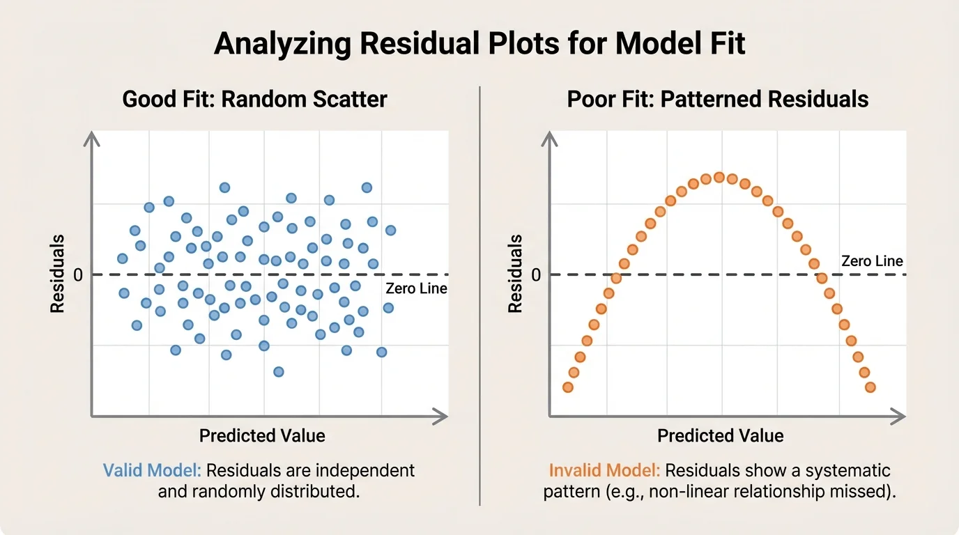
[Figure 4] When scientists compare a model to real data, they often examine the graph first. A good fit means the model predictions follow the general pattern of the observations. But visual similarity is not always enough. Scientists also calculate residuals, the differences between observed values and predicted values.
A residual is calculated as observed value minus predicted value. If a plant model predicts \(15 \, \textrm{cm}\) and the actual height is \(17 \, \textrm{cm}\), then the residual is \(17 - 15 = 2 \, \textrm{cm}\). If another plant was predicted to be \(14 \, \textrm{cm}\) but measured \(13 \, \textrm{cm}\), then the residual is \(13 - 14 = -1 \, \textrm{cm}\).
If residuals are small and scattered randomly around \(0\), the model may be appropriate. If residuals show a pattern, such as starting positive, then negative, then positive again, the model may be missing some important feature of the system.
| Observed value | Predicted value | Residual |
|---|---|---|
| \(17\) | \(15\) | \(2\) |
| \(13\) | \(14\) | \(-1\) |
| \(21\) | \(20\) | \(1\) |
Table 1. Example observed values, predicted values, and residuals for checking model fit.
Residuals are especially helpful because they expose problems that a smooth-looking graph can hide. Later, when judging the strength of a claim, scientists may return to the residual pattern in the graph to decide whether the model was truly capturing the data or just appearing to fit by chance.
Data analysis and computational modeling can go wrong in several ways. One common error is cherry-picking, using only the data points that support a preferred conclusion. Another is confusing correlation with causation. If two variables change together, that does not automatically mean one causes the other.
Another danger is overfitting. This happens when a model is adjusted so closely to one set of data that it captures random noise instead of the true pattern. An overfit model may match existing data extremely well but fail badly when tested on new data.
Ignoring assumptions is also risky. If a motion model assumes no friction, it may work for some situations but fail for rough surfaces. If a chemistry model assumes constant temperature while the reaction actually heats up, the predictions may be inaccurate. In chemistry, for example, a model of carbon dioxide production from a reaction such as \[\textrm{CaCO}_3 + 2\textrm{HCl} \rightarrow \textrm{CaCl}_2 + \textrm{H}_2\textrm{O} + \textrm{CO}_2\] must consider whether temperature, concentration, and gas loss are controlled.
Scientists reduce misuse by documenting methods, sharing data, reporting uncertainty, and testing whether the same model works on independent datasets.
"All models are wrong, but some are useful."
— George Box
This famous statement does not mean models are untrustworthy. It means every model is a simplified version of reality. The goal is not perfection. The goal is usefulness, honesty about limits, and strong reasoning from evidence.
Computational models are central to many fields students encounter in the real world. In climate science, models combine atmospheric data, ocean temperatures, ice cover, and greenhouse gas concentrations to test claims about long-term warming trends. In epidemiology, models help estimate how quickly an illness may spread under different public health strategies. In ecology, models track predator-prey interactions and habitat change.
Engineers use models to test materials, forces, and safety margins before building structures. Medical researchers use models to analyze drug dosage and treatment outcomes. Chemists model reaction rates and concentration changes. In each case, model outputs must be checked against real observations. A prediction alone is not enough.
Even sports science uses data modeling. Coaches analyze movement, heart rate, and recovery time to design training plans. If the data are inconsistent or the model assumptions are poor, the training recommendations may be unreliable. The same scientific principles apply whether the subject is a virus, a river, a bridge, or an athlete.
When using computational models to support a scientific claim, scientists ask several important questions. Were the data collected carefully? Are the variables clear? Are the model assumptions reasonable? Does the model fit the observed data? Are the results repeatable? Are limitations stated openly?
A strong claim sounds like this: The data support the conclusion that the insect population increased by about a factor of \(1.4\) per day over the first four days under controlled conditions. This claim is specific, evidence-based, and limited to the conditions studied.
A weak claim sounds like this: The model proves insect populations always grow by \(1.4\) forever. That statement is too broad, ignores possible limits, and goes far beyond the data.
The best scientific claims are careful without being vague. They are grounded in analyzed data, tested with models, and revised when new evidence appears. That is what makes them both valid and reliable.