A weather app predicts tomorrow's temperature, engineers test airplane designs before building them, and epidemiologists estimate how a disease may spread before hospitals fill up. None of those experts can afford to rely only on guesswork. They use models: simplified representations of reality that can be tested, changed, and improved. When those models are built so that a computer can calculate how a system changes, they become especially powerful.
A computational model is a model that uses calculations, rules, or algorithms to represent a real phenomenon, device, process, or system. A simulation is the running of that model over time or under different conditions so we can observe possible outcomes. Computational thinking matters here because it helps us break a complex problem into smaller parts, identify patterns, represent relationships mathematically, and design step-by-step procedures that a computer can carry out.
For students in grades 9 through 12, the key idea is not just to watch a simulation, but to understand how one is created or revised. Scientists and engineers do not build models once and declare them perfect. They constantly compare predictions to evidence, notice errors, and improve the model. That process is one of the clearest examples of using mathematics and computational thinking together.
A model is a simplified representation of a real object, process, or system. A computational model is a model expressed in a form that a computer can calculate. A simulation is the execution of that model to explore how the system behaves. A variable is a quantity that can change, such as temperature or population. A parameter is a value that shapes the model but is often treated as fixed during one run, such as a growth rate. Assumptions are simplifications made so the model is manageable.
Models are valuable because many real systems are too large, too dangerous, too expensive, or too slow to test directly. You cannot repeatedly crash full-sized cars just to understand every design choice. You cannot wait 50 years to see the long-term effect of a climate policy before making the next decision. A well-designed model lets us test "what if" questions much faster.
Every useful model begins by asking: what exactly is the system, and what are we trying to predict? A model of a roller coaster might focus on speed and acceleration. A model of a cell might focus on chemical concentration. A model of a smartphone battery might focus on charge level, temperature, and power use. The model does not need to include everything. It needs to include the factors that matter most for the purpose of the model.
When building a model, it helps to identify the following parts:
Suppose we want to model the temperature of a greenhouse. As [Figure 1] shows, the system has energy entering from sunlight or a heater and energy leaving through the walls and roof. The output might be indoor temperature. A reasonable first model might ignore wind direction, small shadows, and the exact position of every plant, because those details may not be necessary for the first version.
Choosing what to leave out is one of the most important scientific decisions in modeling. A model that includes every detail becomes impractical to use. A model that ignores too much becomes unrealistic. Good modelers aim for a balance between simplicity and usefulness.
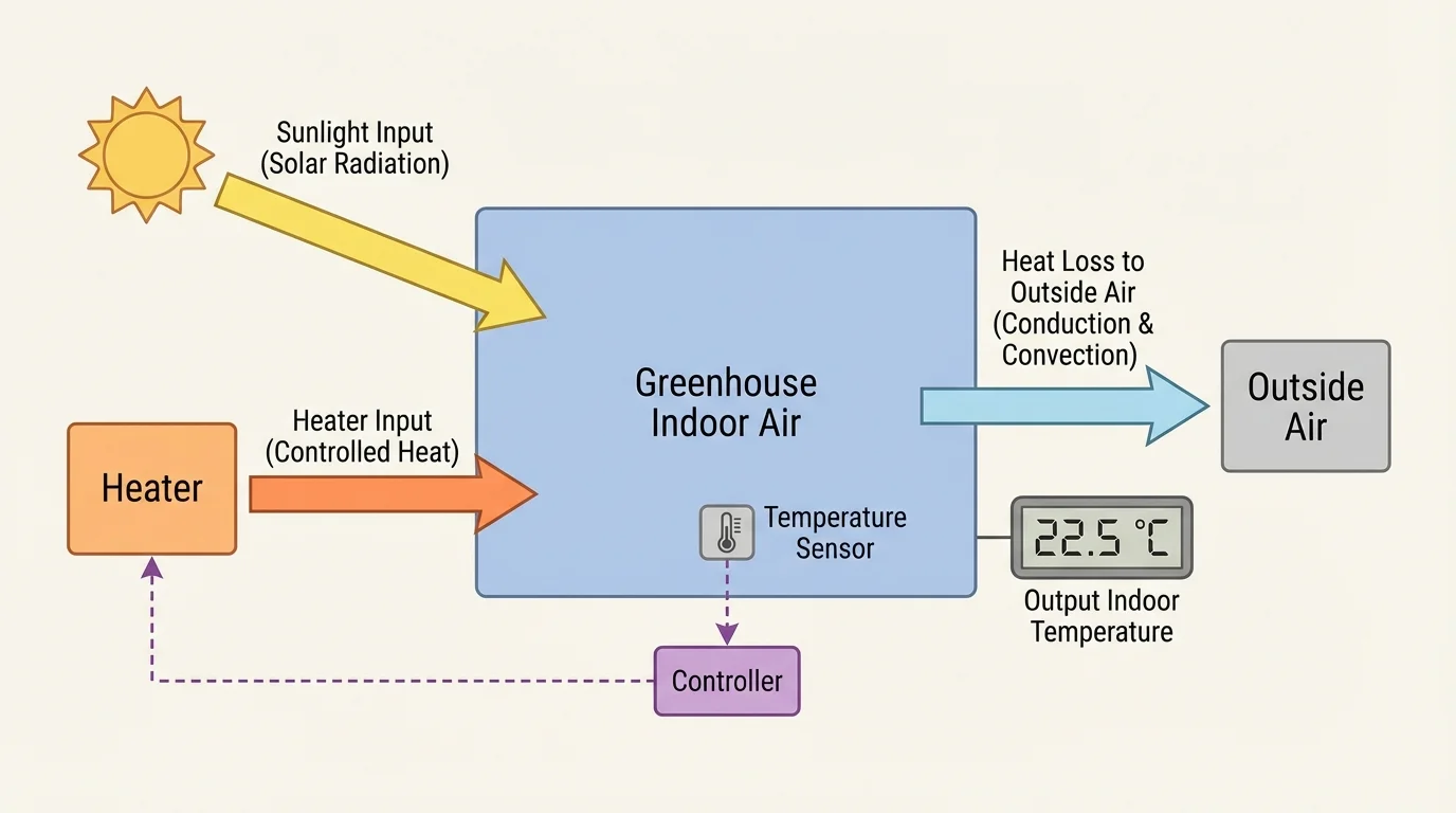
This balance helps define the model's scope. The scope defines what questions the model can answer. A simple greenhouse model may estimate average daytime temperature, but it may not predict temperature at every corner of the room. That is not a flaw if the original goal was only to estimate average conditions.
Earlier work with graphs, functions, ratios, and scientific measurement is essential here. Computational models rely on familiar ideas such as identifying independent and dependent variables, reading trends from data, and using equations to connect quantities.
Assumptions should be stated clearly. For example, a population model might assume unlimited food, constant birth rate, and no migration. Those assumptions may be unrealistic, but they can still be useful if they help isolate one important effect. Later, the assumptions can be revised.
To turn a real process into a working model, we usually translate words into relationships among quantities. This means deciding which variables change and how they affect one another. The relationship can be written as an equation, a rule, a table, or even a set of logical steps.
A very simple population model says the next population equals the current population plus growth. If the population grows by a fraction r each time period, then one discrete model is
\[P_{n+1} = P_n + rP_n = (1+r)P_n\]
Here, discrete model means the model updates in separate steps such as days, months, or years. If a town starts with a population of 100 and grows by 5\% per year, then with \(r = 0.05\), the model gives
\[P_1 = (1.05)(100) = 105\]
and then
\[P_2 = (1.05)(105) = 110.25\]
In real life, population is not usually counted in decimals of a person, which already tells us something important: models often produce mathematically correct values that still need interpretation.
Some models are continuous models, meaning quantities change smoothly rather than in separate jumps. For example, motion under constant acceleration can be modeled continuously with equations such as
\[v = v_0 + at\]
and
\[x = x_0 + v_0 t + \frac{1}{2}at^2\]
If a ball is thrown upward with an initial velocity of \(20\,\textrm{m/s}\) from ground level, using \(a = -9.8\,\textrm{m/s}^2\) and \(x_0 = 0\) gives
\[x = 20t - 4.9t^2\]
At \(t = 2\,\textrm{s}\), the height is
\[x = 20(2) - 4.9(2)^2 = 40 - 19.6 = 20.4 \textrm{ m}\]
Computational models often use these equations repeatedly, especially when many interacting parts make a direct solution difficult.
Deterministic and probabilistic models
A deterministic model gives the same result every time if it starts with the same values and rules. A projectile-motion model under fixed conditions is usually deterministic. A probabilistic model includes chance, so the same starting conditions may lead to different outcomes in different runs. Weather forecasting and some disease-spread models often include probability because real systems contain uncertainty and random variation.
This distinction matters when revising a model. If a deterministic model fails, the equations or assumptions may need correction. If a probabilistic model gives a range of outcomes, then the question is not whether one exact answer is correct, but whether the observed result falls within a reasonable predicted range.
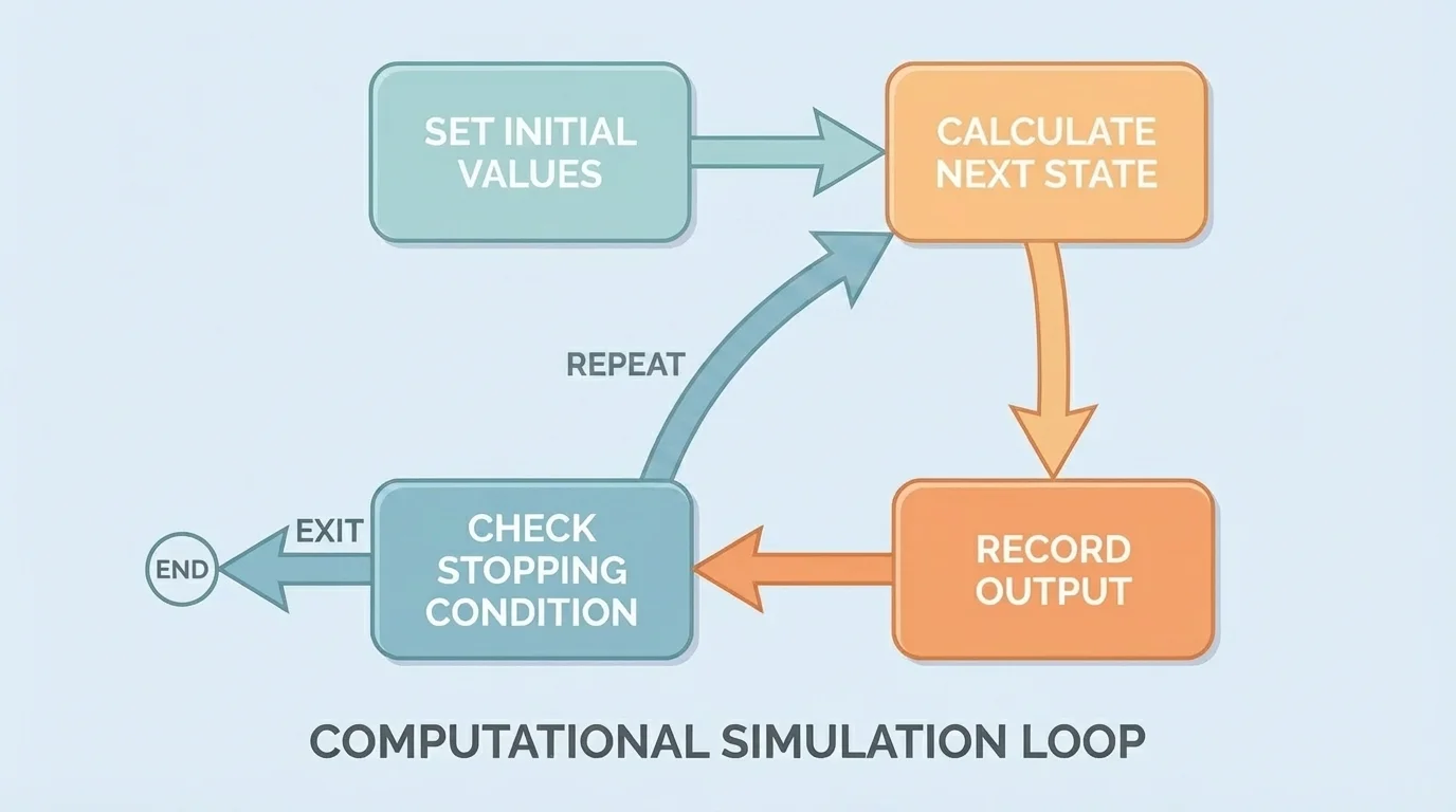
Computers are especially useful when a model repeats the same calculation many times. As [Figure 2] illustrates, a simulation often follows a loop: choose initial values, apply an update rule, store the new result, and repeat until a stopping condition is met. This is where mathematical relationships become computational procedures.
Suppose we simulate the cooling of a hot drink in a room. A simple rule might say that every minute the temperature difference between the drink and the room shrinks by 10\%. If the room is at \(20^\circ\textrm{C}\) and the drink starts at \(80^\circ\textrm{C}\), then the initial difference is \(60^\circ\textrm{C}\). After one minute, the difference becomes \(0.9 \times 60 = 54^\circ\textrm{C}\), so the drink temperature becomes \(74^\circ\textrm{C}\). After another minute, the difference becomes \(0.9 \times 54 = 48.6^\circ\textrm{C}\), so the temperature becomes \(68.6^\circ\textrm{C}\).
The update rule can be written as
\[T_{n+1} = T_{room} + 0.9(T_n - T_{room})\]
With \(T_{room} = 20^\circ\textrm{C}\) and \(T_0 = 80^\circ\textrm{C}\), the computer can apply the same rule over and over. Even a very simple program or spreadsheet can run this simulation for 30 or 60 time steps.
An algorithm is the step-by-step method the computer follows. In a spreadsheet, the algorithm may appear as formulas copied down rows. In code, it may appear as a loop. In both cases, the logic is the same: use the current state to calculate the next state.
Time-step size matters. If the time step is too large, the simulation may miss important behavior. If it is very small, the model may be more accurate but also slower to run. A traffic simulation updated every 10 seconds might miss quick braking events, while one updated every 0.1 second may capture them much better.
Worked example: revising a battery-drain model
A student first assumes a phone battery loses 5\% of its charge each hour. The model is \(B_{n+1} = 0.95B_n\), with \(B_0 = 100\).
Step 1: Run the original model.
After one hour, \(B_1 = 0.95(100) = 95\). After two hours, \(B_2 = 0.95(95) = 90.25\).
Step 2: Compare with observed data.
The real phone is at 88\% after two hours of video streaming, so the model predicts too much remaining charge.
Step 3: Revise an assumption.
The original model assumed constant usage. Streaming uses more power, so a new parameter is chosen: 8\% loss per hour. The revised model is \(B_{n+1} = 0.92B_n\).
Step 4: Test the revision.
Now \(B_1 = 92\) and \(B_2 = 0.92(92) = 84.64\). This is closer to the observed 88\%, though still not exact.
The revised model is not perfect, but it fits the observed situation better because the assumptions match the real conditions more closely.
This example shows a critical idea: revising a computational model is not cheating or "fixing" an answer. It is the normal scientific process of improving a representation so it matches evidence more effectively.
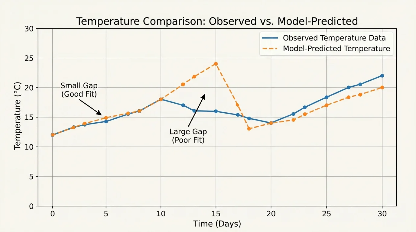
As [Figure 3] suggests, a model becomes meaningful only when its predictions are checked against observations or experimental data. As [Figure 3] shows, validation often involves comparing a graph of predicted values with a graph of measured values. If the lines stay close, the model may be useful. If they separate in a clear pattern, the model likely misses something important.
Validation means checking whether a model represents the real system well enough for its intended use. This is different from simply checking arithmetic. A spreadsheet formula can be calculated perfectly and still describe reality poorly if the assumptions are wrong.
One common way to judge fit is to calculate error, which is the difference between a predicted value and an observed value:
\[\textrm{error} = \textrm{predicted} - \textrm{observed}\]
If a model predicts a room temperature of \(25^\circ\textrm{C}\) and the measured temperature is \(23^\circ\textrm{C}\), then
\[\textrm{error} = 25 - 23 = 2^\circ\textrm{C}\]
Sometimes the size of the error matters more than its sign, so modelers use absolute error:
\[|\textrm{error}| = |25 - 23| = 2^\circ\textrm{C}\]
If the errors are random and small, the model may be acceptable. If the errors all point the same way, the model may be biased. For example, if a temperature model is almost always too low at noon, it may underestimate the effect of sunlight. That pattern gives a clue about how to revise the model.
Revision can happen in several ways:
Sensitivity also matters. A model is sensitive if small changes in one input cause large changes in the output. That can be useful information. If a bridge-design simulation is very sensitive to a material parameter, engineers know that parameter must be measured carefully. If a disease model is sensitive to contact rate, public health planners know social behavior matters strongly.
Some modern climate models divide Earth into many three-dimensional grid cells and repeatedly calculate how energy, air, and water move between them. Even the world's fastest computers still approximate rather than capture every detail of the atmosphere and oceans.
As we saw earlier in [Figure 2], revision does not usually mean rewriting everything from the start. Often, the same simulation loop remains, while one assumption, equation, or parameter changes and the model is tested again.
Computational models appear in nearly every scientific and technical field. Their details differ, but the core process is the same: define the system, choose variables, express relationships mathematically, run the model, compare with data, and revise.
Consider projectile motion. A basic model may ignore air resistance and use only gravity. That model works well for many classroom cases. But for a baseball hit far across a field, drag becomes important. Revising the model to include air resistance usually changes the predicted range. That is a good example of a model becoming more realistic by adding a force that was originally neglected.
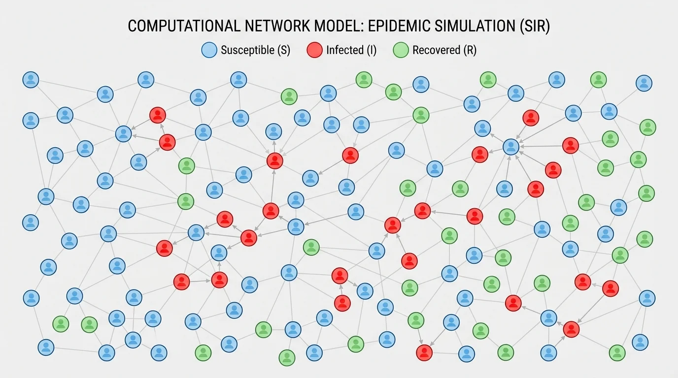
Disease spread offers another important case. In a simple model, people may be grouped as susceptible, infected, or recovered. Contact patterns determine how infection moves through a population. As [Figure 4] illustrates, the structure of who meets whom can change the outcome dramatically. A disease spreads differently in a tightly connected dormitory than in a population where contacts are less frequent.
One very basic disease model can track the number of infected people with a rule such as
\[I_{n+1} = I_n + \textrm{new infections} - \textrm{recoveries}\]
If there are 50 infected people, 12 new infections during one day, and 5 recoveries, then
\[I_{n+1} = 50 + 12 - 5 = 57\]
This is simple, but it already helps show how rates and interactions shape change over time.
Engineers also model designed devices. A thermostat system, for example, uses feedback. If the temperature falls below a set value, the heater turns on; if it rises above the set value, the heater turns off. That kind of model combines mathematics with logical conditions. A simulation can show whether the room temperature stays near the target or swings too widely.
Traffic flow models are another striking example. When one driver brakes, the effect can ripple backward through many cars, causing a "phantom traffic jam" even without an accident. This is a case where many small local decisions create a large system-level pattern. The same kind of systems thinking applies to ecosystems, economies, and electrical grids.
| System | Main variables | Possible assumptions | Reason to revise |
|---|---|---|---|
| Greenhouse temperature | Indoor temperature, sunlight, heater power | Uniform air temperature, constant wall properties | Observed temperatures vary by time of day more than predicted |
| Population growth | Population size, growth rate | Unlimited resources, no migration | Population levels off instead of growing forever |
| Projectile motion | Position, velocity, acceleration | No air resistance | Long-range predictions are inaccurate |
| Disease spread | Susceptible, infected, recovered counts | Equal mixing of all people | Contact network strongly affects spread |
| Battery drain | Charge level, power use | Constant rate of energy loss | Different apps drain power at different rates |
Table 1. Examples of modeled systems, their variables, common simplifying assumptions, and reasons for revision.
The network idea shown again in [Figure 4] is important beyond disease. Information spreading on social media, power failures across a grid, and even rumors in a school can be modeled through connected nodes and interactions.
No model is the real world. That statement sounds obvious, but it is easy to forget when a computer produces detailed graphs and precise numbers. A result like 57.342 does not automatically mean the model is accurate. Precision in output is not the same as truth.
Uncertainty enters in many places: measurement error, missing variables, unpredictable human behavior, and changing conditions. A weather forecast may use enormous amounts of data and still be uncertain because the atmosphere is extremely complex. A school-energy model may fail if windows are opened unexpectedly or if the weather changes suddenly.
Bias can also enter through assumptions. If an algorithm used in public policy is trained on incomplete or unfair data, its predictions may disadvantage certain groups. Responsible modeling requires asking not only "Does this run?" but also "What assumptions shaped it?" and "Who might be affected if it is wrong?"
"All models are wrong, but some are useful."
— George Box
This famous statement does not mean models are untrustworthy. It means every model simplifies reality. The goal is not perfection. The goal is usefulness for a specific purpose. A useful model is one that captures the most important relationships well enough to support understanding, prediction, or decision-making.
When revising a model, the strongest approach is evidence-based. Change one feature, rerun the simulation, compare with data, and judge whether the revision improves the model. That method is more reliable than changing many things at once, because then it becomes hard to know which change mattered.
By building and revising computational models, students learn far more than a technical skill. They learn how science and engineering actually work: through abstraction, mathematics, testing, feedback, and improvement. That is why computational modeling sits at the center of modern research, design, and problem-solving.