Back to the topics list

The significance of a phenomenon is dependent on the scale, proportion, and quantity at which it occurs.

Why Scale, Proportion, and Quantity Change Ecological Meaning

A forest can lose a few trees and remain healthy, but lose the right few trees in the wrong place and an entire stream may warm, fish may disappear, and erosion may spread downstream. That is the central idea of this lesson: the significance of a phenomenon is not determined only by what happens, but by how much happens, what fraction of the system is affected, and at what scale we observe it.

Why the Same Event Can Matter Differently at Different Scales

In ecology, a scale is the level or size at which we examine a phenomenon. A single dead tree may be a minor event for a large forest, but it may be a major event for the insects, fungi, and birds that live on that tree. The same event changes meaning across levels, from organism to biome.

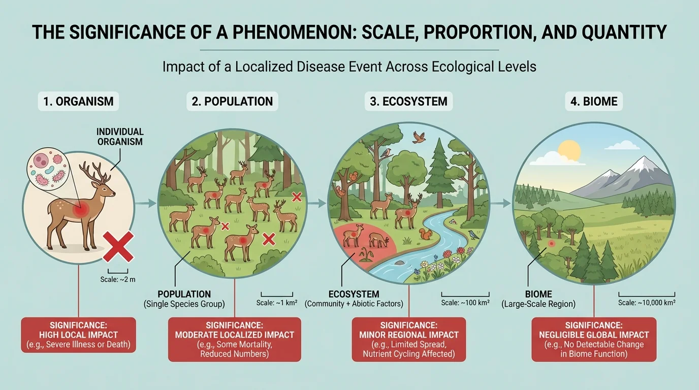
[Figure 1] Ecologists often study several nested levels of ecological organization: organism, population, community, ecosystem, and biome. At the organism level, we may ask whether one deer has enough food. At the population level, we ask whether the deer population is growing or shrinking. At the ecosystem level, we ask how deer grazing changes plants, soil, and streams. At the biome level, we may ask how climate shifts affect forests over huge regions.

A change that looks small at one level can be significant at another. For example, a disease that kills only \(1\%\) of a fish population in one lake may seem minor. But if the disease targets the largest breeding adults, the effect on future reproduction can be much larger than \(1\%\). If the same disease spreads across many lakes, the regional effect becomes much more serious.

This is why scientists avoid judging importance by size alone. A phenomenon becomes significant when its scale matches a vulnerable part of the system. A small oil spill in the open ocean may affect relatively few organisms compared with a spill of the same volume in a salt marsh nursery where many species reproduce. Quantity matters, but location and proportion matter too.

These ideas connect directly to carrying capacity. An ecosystem can support only a limited number of organisms because food, water, space, light, nutrients, and shelter are finite. Whether a population is close to that limit depends on quantity, but whether the limit changes depends on both biotic and abiotic conditions.

Core Ideas: Scale, Proportion, Quantity, and Carrying Capacity

Carrying capacity is not a fixed number permanently attached to an ecosystem. It changes when conditions change. A pond may support \(500\) fish during years with enough oxygen and food, but during a hot summer with low dissolved oxygen it may support far fewer. The important point is that carrying capacity depends on conditions, and those conditions can shift across time and space.

Biotic factors are living influences such as food availability, competition, predators, parasites, and disease. Abiotic factors are nonliving influences such as temperature, water, sunlight, nutrient levels, pH, and fire. Both types affect how many organisms can survive and reproduce.

Proportion often matters more than raw number. Removing \(50\) rabbits from a grassland population of \(5{,}000\) changes only \(1\%\) of the population. Removing \(50\) rabbits from a population of \(80\) eliminates more than half. The same quantity has a very different significance because the proportion is different.

Scale also includes time. A drought lasting \(2\) weeks may stress plants but not destroy a forest. A drought lasting \(2\) years can transform the system by lowering water tables, increasing fire risk, and reducing seedling survival. Duration changes significance just as much as size does.

Biotic Factors and Carrying Capacity

Population density is the number of individuals in a given area or volume, and it strongly influences interactions among organisms. If deer density becomes too high, overgrazing reduces plant biomass, which then lowers future food supply. At low densities, the same number of deer might have little visible effect.

Competition is one major biotic factor. When two species depend on the same limited resource, the significance of competition depends on how scarce that resource becomes. A small overlap in diet may not matter when food is abundant. During a drought or winter shortage, that same overlap can become critical.

Predation also changes carrying capacity indirectly. If wolves reduce elk numbers, browsing pressure on young trees decreases. More trees can survive, which influences shade, soil moisture, bird habitat, and stream temperature. A predator may affect an ecosystem not just by consuming prey, but by reshaping the entire food web.

Disease provides another strong example. A pathogen infecting \(5\) out of \(1{,}000\) individuals might remain localized. But if those \(5\) individuals move frequently, reproduce rapidly, or interact with many others, the outbreak can spread. Significance depends on the proportion infected, the contact network, and the time scale of transmission.

Invasive species reveal how scale can mislead. A few zebra mussels in one part of a lake may seem unimportant. But because they reproduce quickly, filter huge volumes of water, and attach to surfaces, their impact can grow from local to ecosystem-wide. A tiny starting quantity does not guarantee a tiny outcome.

As discussed earlier, the same event can be minor at one ecological level and major at another. That idea helps explain why biotic factors are often studied at multiple scales at once.

Abiotic Factors and Carrying Capacity

Abiotic conditions often set the broad outer limits for life. Water availability is a classic example. A desert may have enough sunlight for plants, but lack of water keeps plant biomass low. Because plant biomass is low, herbivore carrying capacity is also low. One abiotic factor can constrain many levels of the food web.

Temperature matters because it affects metabolism, reproduction, and chemical processes. Warmer water holds less dissolved oxygen. For fish, that means a hot summer can reduce available oxygen just when metabolic demand rises. A temperature increase of only a few degrees may seem small, but its ecological significance can be large if organisms are already near their tolerance limit.

Nutrients such as nitrogen and phosphorus are another major abiotic influence. In small amounts, they support plant and algal growth. In excessive amounts, often from fertilizer runoff, they can trigger algal blooms. When algae die and decompose, bacteria consume oxygen, creating low-oxygen conditions that may kill fish and invertebrates.

Space and habitat structure also matter. A cliff may support only a limited number of nesting birds because safe ledges are scarce. A wetland may support many amphibians only if shallow breeding pools remain long enough for larvae to develop. The amount of suitable habitat, not just total land area, affects carrying capacity.

Abiotic factors can vary across microhabitats. The north-facing side of a hill may be cooler and wetter than the south-facing side. That means carrying capacity can differ over short distances. Ecologists therefore ask not only how much habitat exists, but what proportion of that habitat actually meets a species' needs.

Using Mathematics to Describe Ecological Limits

Ecology uses mathematical representations to make patterns clearer. One simple measure is population density: \(D = \dfrac{N}{A}\), where \(D\) is density, \(N\) is the number of individuals, and \(A\) is area. If a grassland has \(240\) prairie dogs in \(12\) hectares, then \(D = \dfrac{240}{12} = 20\) prairie dogs per hectare.

[Figure 2] Another useful measure is proportion. If \(150\) out of \(600\) trees in a forest stand are infected by a fungus, the infected proportion is \(\dfrac{150}{600} = 0.25\), or \(25\%\). Whether that is serious depends on the species involved, how infection changes survival, and whether the infected trees are clustered or spread out.

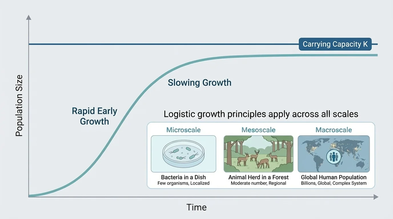
Population growth is often represented by a logistic pattern. When resources are abundant, populations can grow rapidly. As resources become limiting, growth slows and approaches a maximum level called \(K\), the carrying capacity.

A common simplified model is

\[\Delta N = rN\left(1 - \frac{N}{K}\right)\]

where \(\Delta N\) is population change over a time interval, \(r\) is growth rate, \(N\) is current population size, and \(K\) is carrying capacity. The term \(1 - \dfrac{N}{K}\) shows that growth slows as \(N\) approaches \(K\).

Notice what the equation means conceptually. If the population were much smaller, the term \(1 - \dfrac{N}{K}\) would be larger, so growth would be faster. If the population were close to \(300\), growth would slow sharply. This is a mathematical way to show that significance depends on proportion: being \(20\) fish below carrying capacity is very different from being \(120\) fish below it.

Ecologists also use percent change:

\[\textrm{percent change} = \frac{\textrm{new} - \textrm{original}}{\textrm{original}} \times 100\%\]

If a rabbit population drops from \(400\) to \(280\), the percent change is \(\dfrac{280 - 400}{400} \times 100\% = -30\%\). A \(30\%\) decline is often more informative than saying the population lost \(120\) rabbits, because the percentage tells us the loss relative to the original size.

Small Change, Big Effect: Thresholds and Tipping Points

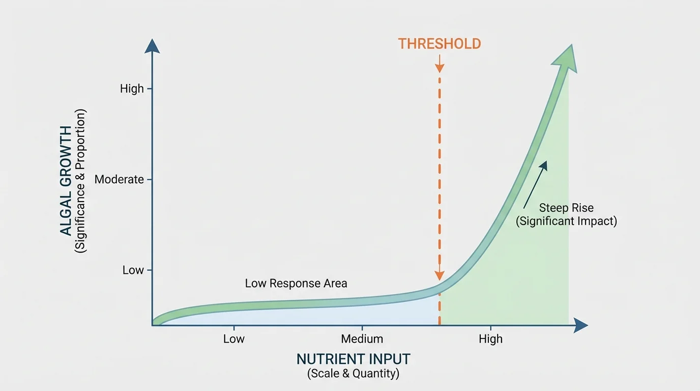
Not all ecological relationships are proportional. Sometimes a small increase in a factor has little effect until a threshold is crossed, and then the system changes rapidly. This is why the significance of a phenomenon may suddenly increase instead of rising gradually.

[Figure 3] A lake can absorb some nutrient input without major visible change. But once nutrient concentration passes a threshold, algae may multiply quickly, light penetration may fall, and oxygen levels may collapse. The quantity added each week may be similar, but the ecological response is not linear.

Forest fires provide another example. A small rise in dead, dry plant matter may not matter much when humidity is high. Under heat, drought, and wind, the same extra fuel can make fire spread explosively. The importance of quantity depends on surrounding conditions.

Feedback loops can amplify change. If warming dries soil, plants may die back. With fewer plants, less shade covers the ground and less water returns to the air through transpiration. That can increase drying further. An initially modest shift becomes more significant through feedback.

This threshold pattern helps explain why environmental monitoring matters. By the time the visible effect is obvious, the system may already have crossed into a much less stable state.

Case Studies Across Scales

Pollinators provide a useful case. A field may still have many flowers even if bee numbers fall slightly. But if bee abundance drops below the level needed to pollinate enough plants, seed and fruit production can decline. In agriculture, that means a modest change in pollinator population can have a large economic and ecological effect.

Algal blooms show how quantity and abiotic factors interact. If fertilizer runoff raises phosphorus in a pond from \(0.01\) parts per million to \(0.03\) parts per million, the increase may seem tiny. Yet in some ponds, that small concentration change is enough to fuel rapid growth. The absolute quantity is small, but the ecological significance is large.

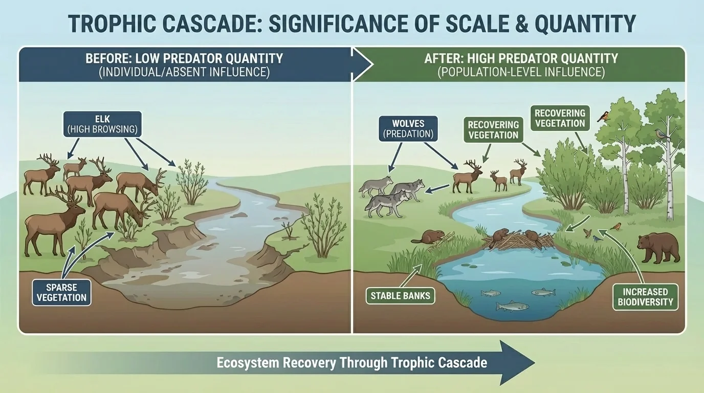
The reintroduction of wolves to Yellowstone is famous because it shows cross-scale effects. Wolves reduce elk browsing pressure, which allows willow and aspen to recover, which changes habitat for birds and beavers and improves stream-bank stability.

[Figure 4] What makes this case powerful is that one population-level change influences many community and ecosystem processes. It is not only the number of wolves that matters, but their proportion relative to prey, their hunting patterns, and the places where they alter herbivore behavior.

Atmospheric carbon dioxide offers the largest-scale example. The concentration of \(\textrm{CO}_2\) in the atmosphere is measured in parts per million, which sounds small. Yet because the atmosphere and climate system operate at planetary scale, relatively small proportional changes in greenhouse gases can alter temperature, rainfall patterns, ocean chemistry, and species distributions worldwide.

Later analysis of the wolf example still returns to the same central idea: predators can matter through chains of indirect effects, not just through direct consumption.

Computational Representations in Ecology

Computational models allow scientists to test what happens when conditions change. A model can estimate how a population responds if rainfall falls by \(15\%\), if predators increase by \(20\%\), or if habitat area is cut in half. This is especially useful when field experiments would take years or would damage a real ecosystem.

Models do not replace field data; they organize it. Scientists use observed values for birth rates, death rates, food supply, migration, and climate, then run simulations across different scales. If a model predicts collapse only when habitat loss exceeds \(40\%\), that threshold helps guide conservation decisions.

Computational representations are important because ecosystems are complex. Many factors interact at once, and humans are not very good at intuitively tracking dozens of connected changes. A well-built model makes hidden relationships visible.

Even simple spreadsheets can reveal patterns. If students record population size over time and graph it, they can see whether growth is roughly linear, exponential, or logistic. Such graphs often show populations slowing as they approach ecological limits.

Why This Idea Matters for Human Decisions

People constantly make choices that depend on scale, proportion, and quantity. Farmers decide how much fertilizer is enough to boost crops without increasing runoff. Wildlife managers decide how many deer a forest can support without severe overbrowsing. City planners decide how much wetland area must be protected to reduce flooding and preserve biodiversity.

Fisheries management is a clear example. Catching \(10{,}000\) fish may be sustainable in a huge, fast-reproducing population but disastrous in a small or slow-growing one. The correct decision cannot come from quantity alone. It must include reproductive rate, population size, habitat conditions, and time scale.

Conservation biology also depends on this principle. Protecting a species in only one small habitat patch may preserve a population temporarily, but if that patch is isolated, genetic diversity may fall and extinction risk may rise. The significance of habitat loss depends on the proportion of habitat lost, the arrangement of what remains, and the movement patterns of the species.

Climate change may be the most important modern example of scale. A change of a few degrees in global average temperature sounds small compared with daily weather swings. But at planetary scale, that shift changes melting rates, storm patterns, drought frequency, ocean currents, and the ranges of many organisms. The quantity appears modest; the significance is enormous.

Understanding ecological significance means asking better questions: How much changed? What proportion changed? Over what area? For how long? At what biological level? Once those questions are asked, patterns that seemed confusing begin to make sense.