If you spin a penny instead of flipping it, will it land heads and tails equally often? Many people guess yes, but real data can surprise you. Probability is not only about what should happen in theory. It is also about what we actually observe when a chance process is repeated many times. That is how mathematicians and scientists build models that describe the real world.
Sometimes the outcomes in a chance process are equally likely, like rolling a fair die. Sometimes they are not equally likely, like tossing a paper cup and watching how it lands. In this lesson, you will learn how to use data to create a probability model, how to decide whether a model is uniform or not, and how to explain why observed data and expected probabilities may not match perfectly.
A chance process is an action with results that cannot be predicted with certainty ahead of time, even if the action is repeated in the same way. Spinning a penny, rolling a die, choosing a marble from a bag, or tossing a paper cup are all chance processes.
Each possible result is called an outcome. For a spinning penny, the outcomes are usually heads and tails. For a tossed paper cup, the outcomes might be open-end up, open-end down, or side.
When we repeat a chance process many times, we collect data. Those data help us estimate how likely each outcome is. A probability model is a list of the possible outcomes and the probability of each one.
Probability describes how likely an outcome is to happen. It can be written as a number from 0 to 1, where 0 means impossible and 1 means certain.
Relative frequency is the fraction or decimal found by dividing the number of times an outcome occurs by the total number of trials.
Uniform model means all outcomes are equally likely. A model that is not uniform has outcomes with different probabilities.
If an event happened 12 times in 50 trials, then its relative frequency is \(\dfrac{12}{50} = 0.24\). That value can be used as an estimate of the probability, especially when the number of trials is large.
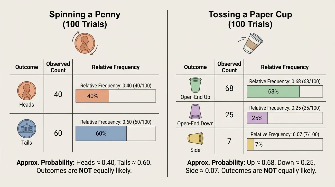
To build a model from data, we start by counting how often each outcome occurs. Then we turn those counts into probabilities using relative frequency. Organized data, like the display in [Figure 1], help us see patterns much more clearly than a messy list of results.
The basic idea is simple. If an outcome appears often, it probably has a higher probability. If it appears less often, it probably has a lower probability. The estimate gets stronger when more trials are included.
The formula for experimental probability is
\[P(\textrm{event}) \approx \frac{\textrm{number of times the event occurs}}{\textrm{total number of trials}}\]
Suppose a spinner is spun 40 times and lands on red 10 times, blue 18 times, and green 12 times. Then the model based on the data is:
These probabilities add to \(0.25 + 0.45 + 0.30 = 1\), as they should in a complete model.
A good probability model has two important features. First, every probability is between \(0\) and \(1\). Second, the probabilities of all possible outcomes add up to \(1\). If they do not, something is wrong with the model.
Relative frequencies do not guarantee the exact true probability, but they are useful estimates. As the number of trials increases, the relative frequencies often settle into a more stable pattern.
A spinning penny is interesting because many people expect heads and tails to be equally likely, but the real test is data. A visual comparison, as shown in [Figure 2], makes it easier to judge whether the two outcomes are close enough to suggest a nearly uniform model.
Suppose students spin a penny 50 times and record the results. They get 27 heads and 23 tails.
The observed frequencies are close, but not exactly equal. Now compute the relative frequencies:
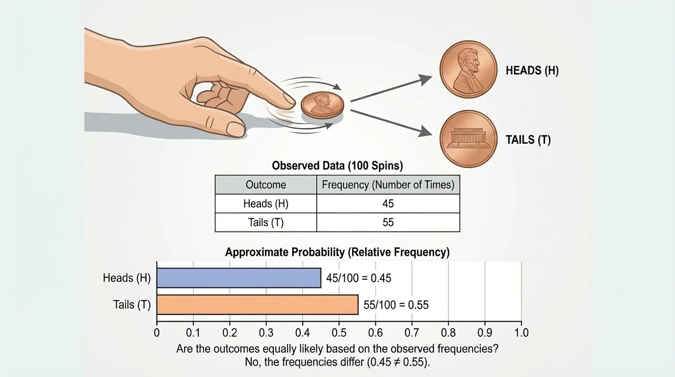
Do heads and tails appear to be equally likely based on these observed frequencies? The best answer is yes—they are approximately equally likely, because 27 and 23 are fairly close. The difference is only 4 out of 50 trials.
However, the data do not show perfect equality. That does not automatically mean the penny is unfair. In a chance process, small differences are expected. Random variation can make one outcome appear a little more often than another, especially in a small or medium sample.
If the penny were spun 500 times instead of 50 times, the relative frequencies might move closer to \(0.50\) and \(0.50\). Looking back at [Figure 2], you can see why bars that are close in height support the idea of a nearly uniform model even when they are not identical.
Observed frequency versus expected probability
Observed frequency is what actually happened in your trials. Expected probability is what your model says is likely in the long run. These are related, but they are not always exactly the same. Probability models are estimates, and repeated experiments can give slightly different results.
If you had no reason to think the penny was unusual, a simple model would be
\[P(\textrm{heads}) = 0.5 \quad \textrm{and} \quad P(\textrm{tails}) = 0.5\]
The observed data of 27 heads and 23 tails are reasonably close to that model, so the model seems acceptable.
A tossed paper cup does not behave like a coin. Its shape, weight, and open end affect how it lands. Because of that, the outcomes often have different probabilities, as [Figure 3] illustrates with unequal bars for the different landing positions.
Suppose a paper cup is tossed 60 times. The results are:
Now find the relative frequencies:
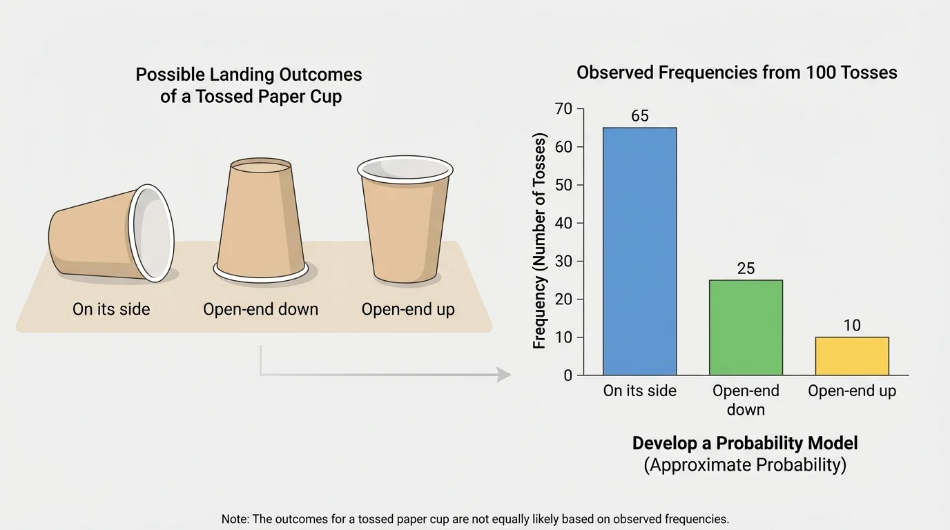
This model is clearly not uniform. The cup lands open-end down much more often than the other ways. That means the outcomes are not equally likely.
This is an important idea in probability. Not every chance process should be modeled with equal probabilities. Real objects can have shapes and physical properties that make some outcomes more common than others. The cup example shows why collecting data matters.
Later, if more tosses are made and the results stay close to the same pattern, the model becomes more convincing. In [Figure 3], one tall bar and two shorter bars suggest a nonuniform model right away.
Once a model is built, it can be used to answer questions. An event may be a single outcome or a group of outcomes.
For the paper cup model above, the probability of landing either open-end up or side is found by adding the probabilities of those two outcomes:
\[P(\textrm{open-end up or side}) = 0.25 + 0.15 = 0.40\]
For the penny model based on 50 spins, the probability of not getting heads is the same as the probability of tails:
\[P(\textrm{not heads}) = P(\textrm{tails}) = 0.46\]
Adding probabilities works when the outcomes cannot happen at the same time in one trial. A spinning penny cannot land both heads and tails on the same spin, so those probabilities can be added for an "or" event.
A fraction, decimal, and percent can all represent the same probability. For example, \(\dfrac{3}{5} = 0.6 = 60\%\). Being able to move between these forms makes probability models easier to read and compare.
Probability models can also be written in a table.
| Outcome | Observed frequency | Estimated probability |
|---|---|---|
| Open-end down | \(36\) | \(0.60\) |
| Open-end up | \(15\) | \(0.25\) |
| Side | \(9\) | \(0.15\) |
Table 1. Probability model for a tossed paper cup based on 60 trials.
Tables are useful because they show the outcomes, the data, and the estimated probabilities all in one place.
Even a good model does not predict exact results every time. If a penny has a model of \(P(\textrm{heads}) = 0.5\), that does not mean you will get exactly 25 heads in 50 spins. You might get 22, 27, or 29.
Differences between a model and observed frequencies can happen for several reasons:
If the agreement between the model and the observed data is poor, we should not ignore it. We should ask whether the model needs to be changed or whether something about the experiment was not fair.
Casinos depend on probability models, but they also know short-term results can be surprising. A game can follow a stable long-run model even while small sets of outcomes look uneven.
For example, if a supposed fair penny gave 80 heads and only 20 tails in 100 spins, that would be much harder to explain as simple random variation. That result would make us question the model or the spinning method.
These examples show how to move from data to a model and then use the model to answer questions.
Worked example 1
A thumbtack is dropped 40 times. It lands point up 11 times and point down 29 times. Build a probability model.
Step 1: List the outcomes.
The outcomes are point up and point down.
Step 2: Find the relative frequency of each outcome.
Point up: \(\dfrac{11}{40} = 0.275\)
Point down: \(\dfrac{29}{40} = 0.725\)
Step 3: Write the model.
\[P(\textrm{point-up}) \approx 0.275 \quad \textrm{and} \quad P(\textrm{point-down}) \approx 0.725\]
This is a nonuniform model because the probabilities are not equal.
This example shows how a real object can behave very differently from a perfectly balanced coin or number cube.
Worked example 2
A spinner is spun 80 times. It lands on yellow 18 times, purple 26 times, and orange 36 times. Find the probability of landing on purple or orange.
Step 1: Estimate each probability from the data.
Yellow: \(\dfrac{18}{80} = 0.225\)
Purple: \(\dfrac{26}{80} = 0.325\)
Orange: \(\dfrac{36}{80} = 0.45\)
Step 2: Add the probabilities for purple and orange.
\(0.325 + 0.45 = 0.775\)
Step 3: State the answer.
\[P(\textrm{purple or orange}) \approx 0.775\]
The event includes two outcomes, so their probabilities are added.
Notice that the answer is greater than either single-outcome probability because the event combines two ways to succeed.
Worked example 3
A penny is spun 20 times on Monday and gives 14 heads. On Tuesday, it is spun 80 more times and gives 38 heads. Use all the data to estimate the probability of heads.
Step 1: Combine the number of heads.
\(14 + 38 = 52\)
Step 2: Combine the total number of spins.
\(20 + 80 = 100\)
Step 3: Find the relative frequency.
\(\dfrac{52}{100} = 0.52\)
Step 4: Write the estimate.
\[P(\textrm{heads}) \approx 0.52\]
Using more trials usually gives a more reliable estimate than using the 20 spins from Monday alone.
Combining data sets is often a smart move because larger samples usually give a better view of the long-run behavior.
Worked example 4
A paper cup model gives \(P(\textrm{open-end down}) = 0.60\), \(P(\textrm{open-end up}) = 0.25\), and \(P(\textrm{side}) = 0.15\). Out of 200 tosses, about how many would you expect to land open-end down?
Step 1: Multiply the probability by the number of trials.
\(0.60 \times 200 = 120\)
Step 2: Interpret the result.
About 120 tosses are expected to land open-end down.
\[\textrm{Expected number} \approx 120\]
This is not a guarantee, but it is a reasonable prediction from the model.
Probability models built from observed frequencies are used far beyond classroom experiments. Engineers test materials over and over to estimate failure rates. Meteorologists study years of weather data to estimate the chance of rain under certain conditions. Sports analysts track free throws, shots, or serves to model performance. Manufacturers test products to estimate how often defects occur.
In all of these cases, the model begins with data. If the data change, the model may need to change too. That is one reason probability is so useful: it gives us a way to make decisions even when outcomes are uncertain.
For example, if a basketball player makes 72 out of 90 free throws in practice, a simple model would estimate the probability of making a free throw as \(\dfrac{72}{90} = 0.8\). Coaches can use that estimate to make strategy decisions, even though they know the player will not make exactly 80% of every small set of shots.
When you use observed frequencies to build a model, always ask careful questions. Were there enough trials? Was the process fair? Were the outcomes recorded correctly? Does the model make sense for the object being tested?
A uniform model is sometimes a good first guess, but real data may show that it does not fit. The spinning penny may look almost uniform, while the paper cup clearly does not. The goal is not to force every situation into equal probabilities. The goal is to let the data guide the model.
That is what makes probability both practical and powerful. We use repeated observations to understand uncertainty, estimate what is likely, and make better predictions about future events.